What are we differentiating, and why?
An X-ray records the result of photons passing through an object. A differentiable model lets us work back from changes in the image to changes in the object or the acquisition.
The idea for this book came from trying to work out what I would give a robotics engineer who wanted to learn differentiable vision. I had a particular reader in mind: someone with a good command of physics and numerical methods, comfortable writing GPU code, who wanted to understand how to infer the arrangement of a scene from an image. Such a reader can follow a derivation and implement it. What they need is a connected account of how the physical model becomes a computation, and how that computation can help them recover something about the world.
I wanted to write that account from first principles. Reaching the interesting part of an explanation only to find it delegated to a library call is a familiar disappointment. Here, the interesting part is precisely the connection between the physics and the implementation. We will build the renderer and its derivatives ourselves, then use them to solve an inverse problem. That should leave us able to make our own modelling choices when the problem changes.
The attraction of differentiable imaging is that a model can help us interpret the discrepancy between what we expected to see and what we measured. Suppose we have an object in approximately the right position. We can render the image our sensor would produce and compare it with an observation. The derivative tells us how that rendered image would respond to a small movement. Combined with the discrepancy, it gives us a way to improve the estimated position. We can also inspect those sensitivities to understand why one movement is easy to detect while another barely registers.
X-ray imaging is the subject of this first volume. It offers an unusually direct starting point because the simplest useful transmission model can be derived from attenuation along a single path. We can understand that calculation in full before extending it to a volume and a detector. Introducing a spectrum changes the relationship between material and signal, while scattering requires us to consider histories that no longer follow a straight path from source to detector. Working through these extensions gives the book a natural progression from a small deterministic calculation to more general photon transport.
Our main application will be finding where a known three-dimensional structure sits relative to an X-ray system. A CT volume acquired before a procedure gives us a representation of the anatomy. During the procedure, a C-arm produces projection images from a source and detector mounted on opposite ends of an arm. We would like to place the volume so that its projection agrees with the observed anatomy. The medical setting supplies a concrete reason to care about the answer, but the underlying task will be familiar to a roboticist: estimate a rigid transform from sensor measurements. Appendix A.1 explains the imaging modalities, and Appendix A.2 introduces the anatomical directions and C-arm conventions.
I assume no medical training. Appendix A exists because knowing the mathematics of imaging does not oblige you to have acquired the vocabulary of radiology by osmosis. It explains what the source produces, what the detector measures and how clinical images are processed. We will return to it whenever those details change the calculation. You should, however, be comfortable with the physics and mathematics expected of an advanced engineering reader, and able to work with PyTorch and CUDA/Warp on an NVIDIA GPU.
The implementation matters to me as much as the derivation. An inverse problem will call its forward model repeatedly, so execution time and memory use directly affect what we can attempt. The code in this book will be written for that use, with the prose doing the explanatory work. Starting from first principles gives us a reason to understand every approximation. It gives us no particular reason to write a poor kernel.
By the end of this volume, I want you to be able to take apart a differentiable X-ray renderer, understand the choices its author made and build one suited to your own problem. Section 1.7 sets out what we will implement and how it will fit together. We will begin with the quantity that the renderer is supposed to predict. Before we differentiate an image, we need to know what its pixels mean.
1.1 Before an image becomes a tensor
A projection radiograph, a fluoroscopic frame and a reconstructed CT slice can all arrive as rectangular arrays. That resemblance is convenient for software and insufficient for physics. A CT volume is a reconstruction from many measurements. A projection records the combined effect of structures along source-to-detector paths. Fluoroscopy adds a temporal setting in which acquisition and processing may depend on earlier frames. Appendix A.1 distinguishes these modalities.
Even within one projection pipeline, several quite different quantities may be called an image. We will keep the distinction in Table 1.1 between the physical field, the detector measurement and the displayed image.
| Quantity | Meaning |
|---|---|
| Optical depth along the path associated with pixel , at photon energy . It is dimensionless. | |
| The corresponding primary transmittance, . | |
| Expected detector signal in a specified measurement domain. | |
| One realised measurement, including the relevant acquisition noise. | |
| A value after image processing or display mapping. |
The first two are properties of a transmission calculation. The remaining quantities involve the detector and, eventually, the processing pipeline. The distinction becomes immediate when we differentiate. Increasing the thickness of a homogeneous attenuating slab reduces primary transmission. Its negative logarithm increases. A display transformation may reverse the visual polarity again. A derivative’s sign makes sense only after we know which quantity was differentiated. Appendix A.5 develops the slab calculation, and Appendix A.15 follows its consequences for differentiable models.
The data labels deserve similar care. In DICOM’s digital X-ray image module, FOR PROCESSING permits detector corrections, while ORIGINAL does not exclude processing such as unsharp masking. Neither label guarantees untouched photon measurements. The relevant transformations have to be recovered from the acquisition and processing information available to us. Appendix A.12 explains the distinction between stored values, image geometry and presentation. [5]
There is a related issue on the volume side. For a conventional CT object whose output units are HU, applying the DICOM rescale slope and intercept converts stored pixel values into Hounsfield units. It does not convert them into a material’s attenuation coefficient at every photon energy. That requires a further model or calibration. A single conventional CT value does not uniquely identify a material spectrum. We will separate those operations when preparing a volume for projection, following Appendix A.11, its discussion of stored values, and the limits of spectral inference from one CT number. [5, 11, 16]
1Object
An attenuation field, before detector noise
Can differ at the same poseMaterial composition or density
2Transport
dimensionless
Primary survival probability
Can differ at the same poseGeometry or material paths
3Detector
counts or charge
Poisson or compound Poisson under the declared event law
Can differ at the same poseSource spectrum, exposure or detector response
Comparison domain in the example below
4Processing
depends on the transform
Noise is transformed, and filtering can correlate pixels
Can differ at the same poseOffset, gain, logarithm or filters
5Display
display values
A display mapping adds no photon observations
Can differ at the same poseWindow, polarity or lookup table
RendererExpected detector counts
Compare in the same domain
ObservationObserved detector counts
Counts are compared here. Comparing processed signals requires modelling their processing and transformed noise. Stored pixels and brightness need not represent counts.
1.2 A model of the measurement
Let contain the quantities we want to vary, and let contain the remaining model inputs. Initially, will describe pose. The CT-derived field, acquisition geometry and exposure model will be held fixed in . Later we may choose to estimate some of those quantities as well.
A deterministic prediction in our chosen comparison domain is
This is the forward problem: supply a possible cause and calculate its consequence. The inverse problem begins with an observation and asks which values of could have produced it. The distinction matters because a perfectly well-defined forward calculation need not have a unique or stable inverse.
To see some of what contains, consider a primary-only model with a point source, stationary anatomy, a single representative ray per pixel and a linear, spatially local detector response. Its expected signal is
Here is the expected open-beam number of photons associated with pixel in the energy interval , over the exposure. is the expected detector output per incident photon, including detection efficiency. Its units determine the units of . The linear attenuation coefficient has units of inverse length, and is the source-to-pixel path expressed in the coordinates of the material field. Dependencies held fixed have been suppressed to keep the equation readable.
Primary means uncollided through the object. The attenuation coefficient accounts for removal by absorption and scattering. Some photons that leave this primary history may still reach the detector after scattering, through paths absent from the equation. Appendix A.4 describes the interactions, and Appendix A.8 explains what the scattered contribution does to the image. [8, 13]
The energy integral is already doing important work. Photons at different energies encounter different attenuation and produce different detector responses. In general, the integral cannot be replaced by an exponential evaluated at one universal effective energy. The source spectrum, transmitted material and detector weighting all matter. Appendix A.3 introduces the source, while Appendix A.6 explains why a clinical exposure is not usually one line integral. [11]
A finite focal spot or detector aperture requires averaging contributions over different paths. Motion requires integration over time. Spatial signal spread requires a detector operator that mixes neighbouring locations. These effects cannot all be hidden inside an object-independent open-beam spectrum. Their geometrical and spatial consequences are developed in Appendix A.7, Appendix A.9 and Appendix A.10.
A measurement also has a distribution. We will write it generally as
The mean alone need not determine that distribution. An ideal count and an energy-integrated signal have different statistics, even when both originate in photon arrivals. If is nonlinear, then generally . Processing an expected detector signal is therefore a particular deterministic approximation to the processed image, not automatically its expectation. Appendix A.9’s treatment of photon and pixel statistics provides the physical background.
For each application, will identify which of these quantities it predicts. We can then choose a comparison with the observed data on intelligible grounds.
Acquired CT
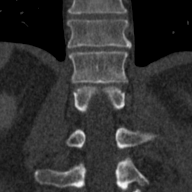
Coronal plane, y=5.81543 mm · −300 to 1,300 HU. x increases right, and z increases up.
Simulated radiograph

Fitting view 1 · 20–55 keV · negative-log display 0–8.
Recovered bone
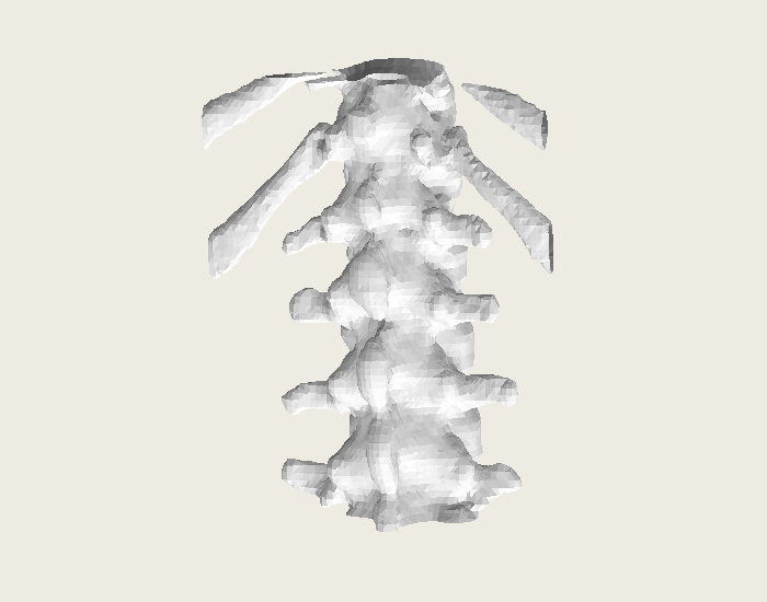
Recorded surface at fraction 0.325 · 1,000 accepted updates.
Rotate the reconstruction and inspect its radiographs. Source data and display rules.
1.3 What a sensitivity image tells us
Imagine translating the anatomy slightly across the beam. Some paths that previously passed mostly through soft tissue now intercept more bone. Others do the reverse. The expected detector signals change in opposite directions on different sides of the projected structures. We can arrange the derivative with respect to that translation as an image, with a signed value at every pixel.
That sensitivity image is the first useful object produced by differentiable rendering. It shows where the projection is responsive to the proposed movement and where it is comparatively indifferent. It need not resemble a radiograph. Its most prominent features may be paired positive and negative bands around anatomical boundaries.
A simplified image-space translation makes the idea explicit. If a smooth projected profile shifts by detector-coordinate units,
A three-dimensional translation in cone-beam geometry is generally more complicated than this uniform image shift. Different depths have different magnifications, and paths through the object change. Nevertheless, the example explains why a motion sensitivity often emphasises structure that the original image merely displays. Appendix A.7 supplies the geometry behind that qualification.
For predicted pixel values and local parameters, the Jacobian is
Each column is one sensitivity image. At a differentiable point, a small perturbation obeys
The product predicts the first-order image change for a combined movement. This is useful before we introduce any optimiser. We can ask whether a particular motion has a visible effect, whether two parameters produce nearly the same effect, or whether a chosen region of the detector contains much information about either.
Now compare the prediction with the observation. For the illustrative least-squares loss
define the residual . The chain rule gives
Each parameter receives a residual-weighted sum of its sensitivity image. Pixels contribute according to how their disagreement would change under that parameter. If moving the model in a given direction increases an already positive residual, that contribution opposes the movement. The gradient accumulates these local effects across the image. Where it is nonzero, a sufficiently small step in the negative-gradient direction reduces this differentiable loss. Recovering the pose will require a sequence of such local decisions, or a more informed optimisation method.
For a general differentiable discrepancy , the image-space factor becomes . Reverse-mode differentiation computes the corresponding vector–Jacobian product without requiring the full Jacobian to be stored. This becomes especially attractive when many material or calibration parameters feed one scalar objective. With only six pose parameters, explicit sensitivities or finite differences may remain competitive for some tasks. The computational choice deserves measurement.
The units remain visible throughout. A sensitivity with respect to a translation measured in millimetres has units of signal per millimetre. A rotational sensitivity has units of signal per radian. Changing the parameterisation changes the numerical gradient, even when the physical family of images is unchanged. We will give those coordinates a proper treatment in Chapter 3.
The six recorded sensitivity images in Chapter 5 make those units and signs visible on the synthetic pelvic example. They sit beside the derivative checks, where we can ask whether the attractive colours correspond to the right calculation.
1.4 Recovering pose
For our running problem, the anatomy is initially represented by a fixed attenuation field in volume coordinates. Pose changes where that field sits relative to the imaging system. Equivalently, we can transform each source-to-detector path into the volume frame and leave the field where it is stored. Rotating the coordinate description should not change the tissue’s attenuation coefficient.
We will use for local coordinates of a rigid pose, with three translational and three rotational degrees of freedom. A rigid transform belongs to . The local coordinates are a way to describe and update it, with a chosen frame and rotation convention. Anatomical projection names do not supply those numerical conventions. Appendix A.2 and its account of C-arm conventions will help us connect the clinical description to the geometry.
The basic estimation problem is
This compact expression leaves room for substantial choices. A likelihood-based discrepancy models the measurement distribution. A feature-based similarity may instead seek structures that remain comparable despite acquisition differences. The first approach needs an adequate statistical model. The second needs an understanding of which information its features retain and discard.
Suppose, for example, that we cannot trust the absolute exposure scale. We might estimate a gain alongside pose, or use a similarity measure insensitive to that gain. Either choice can prevent an irrelevant intensity difference from dominating the fit. It also removes information that might otherwise constrain the solution. An unrestricted per-pixel correction would be able to explain every image at every pose. Nuisance parameters therefore need a physically plausible form and, where appropriate, calibration or regularisation.
Initialisation matters because local sensitivities describe the image near the current pose. They cannot identify a distant correct alignment merely because it exists. The approach developed here therefore needs both a differentiable image calculation for local refinement and a way to obtain a useful starting pose.
DiffDRR expresses Siddon’s projection calculation in vectorised PyTorch operations. DiffPose combines patient-specific pose initialisation with refinement through differentiable X-ray rendering. [22, 23]
The rigid assumption will often be useful for a selected anatomical structure and inadequate for the entire scene. Patient positioning can change the relationship between structures. Contrast material can introduce attenuation absent from the preoperative volume. Instruments may enter the field of view. Appendix A.13, particularly its sections on contrast material and non-rigid anatomy, explains why these are model differences rather than necessarily pose errors. Registration in the presence of anatomical deformation is itself an established research problem. [18]
1.5 When a better fit gives a worse pose
We can make the effect of a model difference precise without introducing a more elaborate renderer.
Let be the true pose in smooth local coordinates. Consider an unconstrained fit with no regularisation, hold any nuisance parameters fixed, and ignore random acquisition noise. Suppose the observation is
where is a small image discrepancy at the true pose. It might contain an unmodelled scatter contribution in a linear detector domain, a calibration error, or the effect of anatomy that changed between acquisitions. We will use pose bias here to mean the systematic displacement caused by this mismatch, without introducing an expectation over repeated measurements.
Linearising the renderer at gives the residual at a small pose displacement:
Let be a fixed, symmetric positive-definite weighting matrix, and define . If has full column rank, minimising the local weighted least-squares problem gives
This is a local, first-order approximation. The inverse is written to expose the dependence, not as advice to form a matrix inverse in an implementation. A substantial displacement would require relinearisation, and rank deficiency requires a different treatment.
The expression explains something an image overlay can conceal. The fit absorbs the component of that resembles a pose-induced image change. In the limiting local case , moving by explains the discrepancy completely within the linearised model. The residual vanishes while the pose moves away from the truth. Conversely, a discrepancy satisfying produces no first-order pose shift, although it remains visible in the image.
Thus the magnitude of an image error is only part of the story. Its alignment with the sensitivity images determines how strongly it can bias pose. This gives us a concrete way to reason about model fidelity. We should be particularly interested in omitted effects that the optimiser can plausibly imitate by moving the anatomy. An optimiser has no loyalty to the patient’s actual position. It has an objective function.
The same calculation shows why some movements are difficult to estimate even with a correct model. If a nonzero perturbation satisfies , it produces no first-order change in the predicted image at the current pose. Nearly null directions produce weak constraints in this local fit. When represents a fixed inverse noise covariance, the weighted sensitivities describe image changes relative to the assumed measurement noise. With a parameter scaling that makes dimensionless, the singular values of express sensitivity in these noise-weighted, scaled coordinates. Millimetres and radians should not be compared by numerical accident.
A single projection of a known three-dimensional object can constrain all six rigid degrees of freedom locally in a suitable geometry. Full column rank is a local condition. It does not rule out a second solution elsewhere, nor does it guarantee useful precision when the columns are nearly dependent. Symmetry, limited field of view and uncertainty in calibration can all undermine the estimate. Adding another view can help when it contributes sensitivity to previously weak directions. The relevant question is what information the additional geometry supplies.
There is a further distinction between the derivative of a fixed acquisition model and the response of an operating imaging system. During fluoroscopy, automatic control can change tube potential, current, pulse width or filtration as attenuation changes. Appendix A.13’s discussion of acquisition control describes this dependence. [17]
Our pose derivative holds fixed. If an acquisition setting instead follows a differentiable response , the total derivative is
A real controller may be discrete or depend on previous frames, so this smooth expression is only applicable where such a response model is appropriate. The fixed-acquisition derivative remains useful. It answers the controlled question we posed, which need not be the same as asking what the C-arm would do during a new acquisition.
Drawn in whitened coordinates for one illustrative pose coordinate
Mixed mismatch
- Fitted pose change δξ
- 1
- Squared weighted residual
- 5 → 1
Parallel mismatch
- Fitted pose change δξ
- 1
- Squared weighted residual
- 4 → 0
Weighted-orthogonal mismatch
- Fitted pose change δξ
- 0
- Squared weighted residual
- 1 → 1
- Mismatch
- Fitted parallel component
- Residual after fitting
Exact constructed example, with true pose at zero. Parallel mismatch admits a perfect fit at the wrong pose. Weighted-orthogonal mismatch remains in the residual.
1.6 Differentiable on paper, in code and in use
Automatic differentiation supplies the chain rule through a computation. Where the recorded operations are differentiable, their derivative rules can be composed to obtain the required gradient. At a kink, a framework may return a chosen subgradient or another convention. A custom backward function contributes the rule its author supplied. PyTorch documents these distinctions explicitly. [24]
This machinery is enormously useful. It also makes it possible to obtain a convincing gradient tensor for an incomplete model. If a calibration step depends on active parameters but has been detached from the computation graph, that dependence is absent from the derivative even if its output affects every pixel. A custom kernel can return a backward result inconsistent with its forward calculation. Floating-point evaluation introduces numerical error. The object of analysis is the mathematical computation represented by those operations and derivative rules, rather than an ordinary derivative of the literal rounded machine map.
The volume representation provides a more instructive example than a catalogue of programming mistakes. Suppose the sampled CT-derived field is treated as piecewise constant in axis-aligned voxels. Siddon’s algorithm computes the line integral exactly for that representation, apart from floating-point error, by finding the relevant path lengths through the grid. The word exactly concerns the voxel model. It makes no claim that the grid captures continuous anatomy exactly. [1]
Alternatively, we might define a trilinearly interpolated field from the samples and integrate it numerically. We have now changed the function being projected. The field is continuous across interior cell faces, but its spatial derivative can jump there. Behaviour at the volume’s exterior depends on the boundary convention. Nearest-neighbour sampling returns us to a piecewise-constant field, whose regions depend on the sample locations and boundary convention. The resulting pose derivatives belong to their respective representations.
Smoothing can make an optimisation landscape easier to traverse. It can also erase information or alter the location of the best fit. Physical blur from a finite focal spot, detector response or motion belongs in the acquisition model when relevant. A smoothing operation introduced to aid optimisation is a numerical choice. Keeping those roles separate will help us interpret coarse-to-fine methods later. Appendix A.10 and the discussion of a frame’s temporal extent give the physical context.
Finite differences offer an independent check on the implemented local derivative. For a scaled direction , we can compare with
Where the directional function is sufficiently smooth, the central difference has second-order truncation error in . Reducing eventually makes subtraction and floating-point error more influential. At a kink, the symmetric difference need not approach either one-sided derivative or the framework’s selected value. A useful check therefore examines an appropriate range of step sizes and understands which regime it is testing.
Agreement establishes consistency between a forward calculation and its derivative over the cases checked. It does not establish that either calculation represents the acquisition accurately. Likewise, convergence of projected images under grid or quadrature refinement does not, by itself, establish convergence of their derivatives. We will examine both as numerical quantities.
The implementation chapters carry this reasoning into CUDA/Warp kernels, explicit reverse operations and Warp tape composition. Reference calculations and derivative checks accompany the relevant algorithms. The arrays remain on the GPU across repeated evaluations, and the optimiser receives only the small control quantities it needs. We will account for the storage and recomputation behind each derivative before deciding what to retain between passes.
Away from the knot: t = 0.25 mm
- CUDA central difference
- Selected CUDA VJP
- Step crosses the knot
Selected VJP: 54.01947 counts/mm. Only h < 0.25 mm stays on this smooth branch. At the smallest steps, rounded count subtraction dominates.
At the knot: t = 0 mm
- CUDA central difference
- Selected CUDA VJP
- Forward one-sided difference
- Backward one-sided difference
Selected VJP: -53.21522 counts/mm. The symmetric difference is zero. The two one-sided limits have opposite signs, so an ordinary derivative does not exist here.
Exact fixture and recorded checks
A single ray passes through a 3 × 3 × 3 field with 1 mm spacing and x weights (1, 2, 1). The base coefficient is the stored FP32 value of 0.02 mm⁻¹. Boundary-sample clamping within the half-cell support gives a 3 mm path and depthfor |t| < 1 mm. The incident mean is 1,000 photons.
The canonical operators use 1,024 samples per ray, FP32 fields/counts and an FP64 pose VJP. Independent scalar FP64 forward checks agree within 0.001 counts. The smooth derivative differs from the independent analytic value by 4.64e-8 counts/mm. This software fixture checks numerical consistency, not physical image accuracy.
1.7 From transmission to transport
We will build one Python package, dpt, and use it to run increasingly demanding image-formation and inverse experiments. The first complete application will take an attenuation volume with declared spatial coordinates, a calibrated source and detector, an observed projection in a specified measurement domain, and an initial rigid pose. It will render a predicted image, evaluate its disagreement with the observation, and use derivatives to update the pose. Its outputs will include the estimated transform and a record of the fit. In controlled recovery experiments, we will also measure error against a known pose: an attractive overlay is a rather generous unit test.
We will first complete this application with a deterministic primary-transmission model. That gives us a working renderer and pose-recovery loop to extend when we introduce energy dependence, detector effects and scattered histories. We can then examine how each change to the measurement model affects the recovered pose.
The first complete application
We begin in the middle of the eventual renderer, with a known optical depth. That lets us check the conversion from attenuation to signal before a coordinate error can impersonate a physics error.
- In Chapter 2, we implement
dpt.transmission.transmit. It takes one optical depth per detector pixel and, when requesting expected counts, an open-beam expectation. It writes primary transmission, expected counts or log transmission to caller-owned device arrays. We also derive and independently check its local derivatives. The early experiments supply optical depths from specified slabs and numerical test cases, and they do not yet form an image from a volume. - Chapter 3 defines the source, detector pixel centres, coordinate frames and rigid-pose updates. From those definitions we construct source-to-detector rays in the volume’s coordinates. The output of this stage is geometrical: it tells us where to evaluate the material field, but has not yet accumulated attenuation.
- In Chapter 4, we represent the sampled attenuation field, intersect rays with its support and integrate along the physical paths. This produces the optical-depth array that Chapter 2’s transmission operation consumes. We now have the first volume-to-image renderer. We test it against independently known path integrals and examine convergence as the numerical resolution changes.
- Chapter 5 connects derivatives through pose, coordinates, sampled fields, path integration and transmission. A correct derivative of the exponential alone is not a pose gradient. The assembled derivative must agree with independent perturbation checks. Interpolation and support boundaries need particular attention.
- Chapter 6 adds an objective in the chosen comparison domain and a driver that repeatedly renders, differentiates and proposes pose updates. The volume and reusable buffers stay on the GPU across those iterations. Recovery experiments start from controlled initial poses and report pose error as well as image disagreement.
How the package fits together
The scientific implementation lives under python/dpt/. The modules in Table 1.2 are present in the accompanying library, and the chapter order describes how we arrive at their design. You can follow that argument from transmission onwards, or use the map to find the operation needed for an experiment.
| Package area | Responsibility | Where we build it |
|---|---|---|
dpt.transmission | Convert optical depth into primary signal and propagate its output sensitivities. | Chapter 2. |
dpt.geometry, dpt.volumes, dpt.projection | Describe frames and sampled fields, construct finite paths and accumulate optical depth. | Chapters 3–4. |
dpt.autodiff | Manage a first-order derivative pass and the lifetime of its saved inputs and cotangents. | Chapter 5. |
dpt.objectives, dpt.recovery, dpt.registration | Form a loss and its image seed, compose the renderer’s reverse pass and choose pose updates. | Chapter 6. |
dpt.spectral_recovery, dpt.spectral_inputs | Fit a shared pose and declared calibration groups across supplied views, and keep evaluation views outside the fit. | Chapter 7, using Chapter 8’s operators. |
dpt.materials, dpt.material_projection, dpt.spectral, dpt.detector | Project material paths, sum their energy-dependent transmission and apply the chosen detector model. | Chapter 8. |
dpt.transport, dpt.stochastic_recovery | Score random histories, estimate supported derivatives of their expected signal and make inverse updates with independent batches. | Chapters 9–10. |
dpt.validation, dpt.experiments | Check operators against independent references and record the inputs, source and outputs of an execution. | Throughout the implementation. |
For the first pose fit, PrimaryPoseEvaluator connects project_optical_depth() to transmit(), then passes the predicted counts to evaluate_objective(). The objective writes both a scalar loss and an image-sized derivative seed. transmission_vjp() turns that seed into sensitivities with respect to optical depth, and projection_vjp() carries them back to pose. This is the chain behind the compact forward model in Section 1.2. Chapter 6 follows the complete call sequence after we have built and checked its parts.
The objects have different lifetimes. GridSpec and DetectorGeometry describe the fixed field lattice and acquisition geometry. A specification such as TransmissionSpec selects an operator’s configuration, and its prepare_* function allocates reusable workspace on an explicitly chosen CUDA stream. The evaluator owns the image buffers connecting the operations. It prepares them once, then reuses them while the optimiser proposes new poses. PoseChart defines how six scaled optimiser coordinates produce a rigid transform. That chart stays fixed while L-BFGS retains differences between earlier iterates, because those differences must share a coordinate system.
Preparation keeps allocations out of repeated device evaluation, but it does not remove every transfer. The recovery controller reads the scalar loss, a small gradient and status values before proposing its next trial. The volume and image buffers stay on the device. When a derivative recomputes a ray instead of saving all its samples, the original field and pose must remain unchanged until that reverse pass has finished. These ownership rules explain much of the machinery surrounding what may look, at first, like a modest exponential.
An executable experiment under experiments/ prepares inputs, calls the package and records its outputs. projection-convergence/ separates quadrature error from field discretisation, while projection-gradients/ checks the reverse calculation over a range of perturbation sizes. pose-recovery/ then runs the assembled inverse problem on a declared analytic field. Its target comes from the same discrete renderer at a known pose, so recovery measures consistency of that software experiment. Physical validation needs independently supplied acquisitions and a defensible material model.
The book’s listings are extracted from marked regions in those canonical source files. A listing’s number locates the discussion, and its source link identifies the implementation and line range. Experiment records retain the configuration, source snapshots and output checksums needed to trace a numerical result back to its execution. Later figures can draw those recorded arrays in the book’s visual style without acquiring a second implementation of the physics.
Extending the measurement model
With pose recovery working, Chapter 7 introduces controlled exposure, gain and offset changes, then examines how a pose fit responds to those changes and to errors in its scene model. Chapter 8 then implements energy-dependent materials, spectral integration and detector response. Spectral experiments require those operators, and scatter experiments must also wait for Chapter 9’s transport implementation. The distinctions in Appendix A.13 will become modelling choices rather than background reading.
Chapter 9 adds free flights, interactions and detector scoring, giving us a richer account of photon histories. In a detector domain where the response is linear, expected primary and scattered contributions can be added. After nonlinear processing, the corresponding image values generally cannot. Tracking this distinction from the beginning will make the extension less abrupt.
Stochastic transport also introduces a second source of randomness into our work. The acquisition is noisy because the physical measurement is random. A Monte Carlo estimate of an expected signal is noisy because we have evaluated only a finite sample of simulated histories. Increasing that sample can reduce numerical estimation variance. It does not retrospectively increase the number of photons in the patient’s recorded exposure.
When we differentiate a stochastic estimator, we must ask whether it estimates the derivative of the intended expectation. Parameter-dependent sampling and moving discontinuities make that a mathematical problem in its own right. Chapter 10 implements density derivatives on a fixed grid and derivatives of source amplitude, then uses independent batches in an expected-signal inverse problem. Moving-boundary derivatives require additional estimator terms and remain outside this implementation. The deterministic pose derivative from Chapter 5 cannot simply be carried through a sampled collision history. The distinction between photon statistics and pixel statistics will remain useful throughout.
This volume concerns image formation and the inverse problems built upon it. An image fit is not a clinical validation, and a detector signal is not absorbed dose. Readers interested in those radiation quantities should begin with Appendix A.14.
For now, we need one path through an attenuating object. We will work out what reaches the detector, then move the object and work out what changes. That small calculation is the beginning of the renderer.
References
- Gopalakrishnan, Vivek and Golland, Polina (2023). Fast Auto-differentiable Digitally Reconstructed Radiographs for Solving Inverse Problems in Intraoperative Imaging. Clinical Image-Based Procedures, 13746, 1-11. Cham: Springer. https://doi.org/10.1007/978-3-031-23179-7_1
- Gopalakrishnan, Vivek, Dey, Neel and Golland, Polina (2024). Intraoperative 2D/3D Image Registration via Differentiable X-ray Rendering. Proceedings of the IEEE/CVF Conference on Computer Vision and Pattern Recognition, 11662-11672. https://doi.org/10.1109/CVPR52733.2024.01108
- DICOM Standards Committee (2026). DICOM PS3.3 2026c: Information Object Definitions. National Electrical Manufacturers Association. https://dicom.nema.org/medical/dicom/current/output/chtml/part03/PS3.3.html
- Alvarez, R. E. and Macovski, A. (1976). Energy-selective reconstructions in X-ray computerised tomography. Physics in Medicine and Biology, 21(5), 733-744. https://doi.org/10.1088/0031-9155/21/5/002
- Schneider, Uwe, Pedroni, Eros and Lomax, Antony (1996). The calibration of CT Hounsfield units for radiotherapy treatment planning. Physics in Medicine and Biology, 41(1), 111-124. https://doi.org/10.1088/0031-9155/41/1/009
- Hubbell, J. H. and Seltzer, S. M. (1995). Tables of X-Ray Mass Attenuation Coefficients and Mass Energy-Absorption Coefficients 1 keV to 20 MeV for Elements Z = 1 to 92 and 48 Additional Substances of Dosimetric Interest. Gaithersburg, Maryland: National Institute of Standards and Technology. https://doi.org/10.6028/NIST.IR.5632
- Siewerdsen, Jeffrey H. and Jaffray, David A. (2001). Cone-beam computed tomography with a flat-panel imager: Magnitude and effects of x-ray scatter. Medical Physics, 28(2), 220-231. https://doi.org/10.1118/1.1339879
- Otake, Yoshito, Wang, Adam S., Stayman, J. Webster, Uneri, Ali, Kleinszig, Gerhard, Vogt, Sebastian, Khanna, A. Jay, Gokaslan, Ziya L. and Siewerdsen, Jeffrey H. (2013). Robust 3D–2D image registration: application to spine interventions and vertebral labeling in the presence of anatomical deformation. Physics in Medicine and Biology, 58(23), 8535-8553. https://doi.org/10.1088/0031-9155/58/23/8535
- Rauch, Phillip, Lin, Pei-Jan Paul, Balter, Stephen, Fukuda, Atsushi, Goode, Allen, Hartwell, Gary, LaFrance, Terry, Nickoloff, Edward, Shepard, Jeff and Strauss, Keith (2012). Functionality and operation of fluoroscopic automatic brightness control/automatic dose rate control logic in modern cardiovascular and interventional angiography systems: A Report of Task Group 125 Radiography/Fluoroscopy Subcommittee, Imaging Physics Committee, Science Council. Medical Physics, 39(5), 2826-2828. https://doi.org/10.1118/1.4704524
- PyTorch contributors (2026). Autograd mechanics. PyTorch documentation. https://docs.pytorch.org/docs/2.14/notes/autograd.html
- Siddon, Robert L. (1985). Fast calculation of the exact radiological path for a three-dimensional CT array. Medical Physics, 12(2), 252-255. https://doi.org/10.1118/1.595715