Coordinate frames and the geometry of motion
Moving an object changes where source-to-detector rays pass through it. To calculate that change, we need coordinate frames, physical pixel locations and an unambiguous account of where the object rotates.
Now let’s ask our renderer to rotate a vertebra about its centre. That centre should stay at the same detector location while the surrounding bone changes its projected shape. Rotate about the X-ray source instead, and the centre moves across the image. Both calculations can use a perfectly valid rotation matrix. The difference is where the rotation acts.
Chapter 2 gives the change in transmission caused by a change in the material along a path. A pose derivative also needs to know which path a movement produces. If a translation is expressed in the wrong frame, the derivative can be numerically impeccable and point in the wrong physical direction. Automatic differentiation is quite willing to help with this.
We need to connect a detector array entry to a finite line segment through the object, then describe how that segment changes with pose. The attenuation field lives in physical object coordinates. Pixel indices, source locations and optimisation parameters must reach those coordinates through a chain whose directions and units we can inspect.
This gives the next part of the library introduced in Chapter 1: dpt.geometry. Its small host objects describe the acquisition and pose. The projector will copy their fixed metadata into its prepared CUDA workspace, then construct rays on the device. We are establishing the inputs from which Chapter 4 will compute the optical depths that transmit() already knows how to consume.
3.1 Naming and framing
A frame specifies an origin and three orthonormal axes. A point exists independently of the frame, but its three coordinates depend on that choice. We write for the column vector containing a point’s coordinates in frame . The superscript names the frame. It is not a power.
We use the four frames defined in Table 3.1. All are right-handed, with positive third axis given by the cross product of the first two. Physical coordinates and translations are in millimetres, and angles are in radians.
| Frame | What it is attached to | Origin and axes |
|---|---|---|
| , world | The fixed reference for the acquisition | A declared physical origin and basis, shared by the source, detector and object poses. |
| , object | The rigid anatomy or volume | A fixed origin and basis in which the attenuation field is defined. Coordinates are physical distances, not voxel indices. |
| , source | The ideal point source | Origin at the focal point. Calibrated axes describe source orientation when the emission model needs it. |
| , detector | The detector plane | Origin at the geometric centre of the active rectangle. First axis follows increasing column index, second follows increasing row index. |
The detector’s third axis follows from handedness. Its sign relative to the source is a calibration choice, not a consequence of calling the frame right-handed. In our centred examples the source lies on the negative side of that axis. A tilted or offset acquisition will be represented by its actual source position.
A rigid transform maps coordinates from frame into frame :
O moves with the solid. Changing the world frame changes its coordinates.
Coordinates are in millimetres.
Choosing a world frame does not move the apparatus. For patient coordinates we can use the left, posterior and superior (LPS) axes described in Appendix A.2. A detector-centred acquisition frame is also possible. The conversion between these choices must be explicit: a label such as “world” supplies no anatomical orientation on its own.
3.2 Rigid transforms and their inverses
Let contain the three axes of frame , expressed as columns in frame , and let be the position of the origin in . A point transforms as
The orthogonality condition preserves lengths and angles. The determinant condition excludes a reflection, which would otherwise satisfy the same orthogonality test. Translation changes the coordinates of the origin but leaves displacements between points unchanged.
We can put rotation and translation into one matrix by appending a homogeneous coordinate of one to a point:
These rigid-transform matrices form , the special Euclidean group. Their products and inverses remain rigid transforms.
For a displacement or ray direction , translation cancels when we subtract its two endpoints. Its homogeneous coordinate is zero:
Adding the translation to a direction makes that direction depend on the chosen origin.
To invert the point transform, subtract and multiply by . The inverse is therefore
The inverse translation is expressed in frame . Simply negating the original translation leaves it in the wrong basis whenever the frames are rotated relative to each other.
For a chain from through to , substitution gives
The rightmost transform acts first on a column vector. Matching adjacent frame labels make the intended chain readable: enters, is intermediate, and leaves. Reversing the multiplication changes the motion and usually makes the labels incompatible as well.
Changing a point’s coordinate description is a passive use of a transform, while physically moving the object while holding the world fixed is an active use of the same matrix algebra. To specify the latter, we change while keeping the source and detector poses fixed.
RigidTransform makes these distinctions visible at the call site. point() includes translation, while direction() cannot accidentally inherit it. The same class describes any declared rigid map, but the projector takes its object-to-world instance. The code calls that map T_WO: it is exactly the transform denoted by in the prose. The code’s letter T in this name carries no transmission meaning.
@dataclass(frozen=True, slots=True)
class RigidTransform:
    """T_WO maps object points into world coordinates; translation is in mm."""

    rotation: Matrix3 = IDENTITY
    translation_mm: Vector3 = (0.0, 0.0, 0.0)

    def __post_init__(self) -> None:
        object.__setattr__(self, "rotation", rotation_matrix(self.rotation))
        object.__setattr__(self, "translation_mm", vector3(self.translation_mm, "translation"))

    def point(self, point_mm: Vector3) -> Vector3:
        rotated = matvec(self.rotation, point_mm)
        return cast(Vector3, tuple(rotated[i] + self.translation_mm[i] for i in range(3)))

    def direction(self, direction: Vector3) -> Vector3:
        return matvec(self.rotation, direction)

    def inverse(self) -> RigidTransform:
        inverse_rotation = transpose(self.rotation)
        translation = matvec(inverse_rotation, self.translation_mm)
        return RigidTransform(inverse_rotation, cast(Vector3, tuple(-x for x in translation)))

    def compose(self, right: RigidTransform) -> RigidTransform:
        """Return self @ right; the right-hand map is applied first."""
        return RigidTransform(
            matmul(self.rotation, right.rotation), self.point(right.translation_mm)
        )

    def packed(self) -> tuple[float, ...]:
        """Twelve float64 device values: row-major rotation, then translation."""
        return (*self.rotation, *self.translation_mm)
The immutable object checks the rotation’s handedness and orthonormality when it is constructed. That check protects the transpose-as-inverse calculation on which every subsequent ray depends. packed() stores nine row-major rotation entries followed by three translation entries in binary64. Row-major storage says how to address the coefficients, and they still act on column vectors. The constant fourth row of the homogeneous matrix need not travel to the GPU at every trial pose.
These Python methods handle calibration and a handful of pose coordinates. They do not perform the per-pixel ray calculations. The CUDA projector applies the same inverse map inside each ray’s execution, using the prepared geometry and the current twelve-value pose buffer.
3.3 Detector coordinates and pixel centres
Let the detector have columns and rows. We follow Appendix A.12: is the zero-based column index, the zero-based row index, and an array stores the sample at . Let and be the positive detector pitches along those two directions, in millimetres.
For our detector-centred frame, the physical position of pixel centre is
The half-index offsets follow by placing the first and last centres symmetrically about zero. We model contiguous rectangular pixel cells extending half a pitch on either side of each centre. Their footprint has width and height . For an odd number of columns, the central column lies at zero. For an even number, zero lies halfway between the two middle columns. Adding a further half pixel would shift every ray.
4 columns × 3 rows · detector frame D
Pixel centreCell boundary
Centre of pixel (1, 1) in D
Choose a centre or use the selector. On the grid, arrow keys move one pixel. ↑ increases j.
- Column pitch Δc
- 0.4 mm
- Row pitch Δr
- 0.6 mm
- First centre (0, 0)
- (−0.6, −0.6, 0) mm
- Last centre (3, 2)
- (0.6, 0.6, 0) mm
Cell edges extend to x = ±0.8 mm and y = ±0.9 mm. Every centre has z = 0.
For example, a detector with four columns, three rows and pitches and has the pixel centres listed in Table 3.2.
| Pixel | Horizontal position in (mm) | Vertical position in (mm) |
|---|---|---|
The unequal pitches are a neat trick to make an accidental row/column exchange visible, in a way a square array with equal spacing would not. The detector pose then places each centre in the world:
Equivalently, if calibration supplies the first pixel centre and unit directions and , we can write
These are the same geometry with different origins. With the centred convention, the basis vectors are the first two columns of , and the first pixel centre follows by evaluating the centred formula at .
DetectorGeometry stores the second form. Its origin_mm is , the first pixel centre, while the origin of frame in Table 3.1 is the rectangle’s geometric centre. Starting from a centred calibration, obtain origin_mm by subtracting half the first-to-last column span along the column basis and half the first-to-last row span along the row basis from the centre’s world position. Apply that conversion once. The ray kernel then only adds integer multiples of the two calibrated pitch vectors.
The descriptor’s u and v are the world-space column and row unit vectors. spacing_mm orders column pitch before row pitch, whereas shape orders rows before columns, like the stored image. The deliberately different orders follow physical coordinates and array indexing respectively. Construction rejects nonpositive pitches, nonorthogonal detector axes and a source in the detector plane, where our perspective ray construction would be degenerate. A flattened pixel uses row * width + column, so the image returned by transmission retains this same ordering.
For ray construction, the pitches belong to the calibrated detector plane. DICOM’s Imager Pixel Spacing measures image-pixel separation at the front plane of the detector housing. Pixel Spacing can instead encode a patient-depth magnification correction or a fiducial calibration. Select the spacing and plane together: substituting the patient-calibrated value into a detector-plane model changes the projection geometry. [5]
The geometric centre of the rectangle need not be the principal point. Here the principal point means the perpendicular projection of the source onto the detector plane. If the source in detector coordinates is , with , that point is . Its continuous pixel coordinates are
An offset principal point belongs in the calibrated geometry. It does not require redefining the detector’s array centre. Likewise, the normal separation and the distance from the source to the detector’s geometric centre coincide only for a centred source.
3.4 Constructing source-to-detector rays
The source-frame origin is the focal point, so its world position is . For one pixel, abbreviate and use its centre as the detector sample. Their difference gives a direction and a finite source-to-pixel distance:
The hat marks a unit vector. With physical distance measured from the source, the ray segment is
At we recover the source, and at we recover the detector sample. Material behind the source or beyond the detector does not belong to this segment. The part inside the object will be selected by intersection with its physical support.
We can also interpolate directly between the endpoints with a dimensionless parameter :
The factor converts a step in into a physical distance. A normalised ray direction alone does not supply this factor when the integration parameter still runs from zero to one.
To evaluate an attenuation field stored in object coordinates, transform both endpoints with :
Subtracting the endpoints cancels translation. Orthogonality then gives
A rigid change of frame preserves the distance element. If is the attenuation field in object coordinates, extended by zero outside the modelled object, the optical depth is
Here has units , so is dimensionless. Any additional attenuating structure, such as a table, needs its own contribution if it is part of the forward model. The open-beam count remains the detector-defined quantity from Chapter 2, and ray construction adds no second inverse-square factor.
One ray through each pixel centre retains Chapter 2’s spatial approximation. To average over a finite pixel or source spot, construct more source-to-detector samples with the same coordinate rules and average their transmitted contributions. The averaging weights combine the detector contributions, while physical distance determines the attenuation accumulated along each ray.
3.5 Move the object or move the acquisition
Suppose the source and detector stay fixed while the object moves. The object-frame field stays attached to the anatomy. For a pose with rotation and translation , its value at a world point is
The inverse pose finds which object point occupies the queried world position. Moving the ray endpoints into therefore lets us sample the original field. Repeatedly rotating and resampling the voxel array would introduce an interpolation operation at every pose change, with a different numerical effect from querying the same field along new paths.
The transforms that the ray calculation needs are the source and detector poses relative to the object:
This also explains why a common rigid change of world coordinates leaves the geometry unchanged. Premultiply every world pose by the same rigid transform . Then
and the same cancellation holds for the detector. The unchanged ray in object coordinates produces the same optical depth and transmission.
Let the object’s old and new world poses be and , and define the world-space displacement . Instead of moving the object to , keep it at and transform the acquisition by the inverse displacement:
The final identity proves equality of both relative poses. For a pure object translation to the right, the equivalent acquisition translation is to the left. A rotation requires transforming the source and detector together about the prescribed centre. Rotating the detector alone changes the acquisition.
The two constructions predict the same primary signal when the relative geometry, object field and open-beam measurement model are the same. Moving a real C-arm, however, need not preserve those conditions. Automatic exposure control may adjust the X-ray output, requiring an updated open-beam count and, if the spectrum changes, an updated spectral model. The new rays may also pass through different lengths of a stationary table, changing the table’s contribution to optical depth. Matching the source and detector poses relative to the anatomy does not by itself account for either effect.
When both the object and acquisition poses are unknown, these measurements cannot distinguish a shared rigid motion from no motion at all: only their relative geometry matters. We therefore hold one reference pose fixed while fitting the others. Without that constraint, different pose combinations define identical rays, leaving the optimiser free to move through parameter space without changing the predicted image.
3.6 Pose parameters and local updates
A rigid pose has three translational and three rotational degrees of freedom. Its matrix representation stores more entries, with constraints on the rotation. We need a way to update a valid pose while retaining a valid rotation. Table 3.3 compares the constraints imposed by common rotation representations.
| Rotation representation | Stored values | What an update must respect | Active clockwise quarter-turn about , viewed from towards the origin |
|---|---|---|---|
| Rotation matrix | Nine entries | Orthogonality and determinant . Adding arbitrary entries breaks these constraints. | , acting on column vectors. |
| Euler angles | Three angles | A declared axis order and fixed- or moving-axis convention. Singular configurations depend on that choice. | for fixed-axis , then , then rotations: . |
| Unit quaternion | Four components | Unit norm, declared component order, and the fact that and describe the same rotation. | in order, using the Hamilton convention with . |
| Local rotation vector | Three components | Axis given by direction, angle by length, and a fresh increment is composed with the current rotation. | , giving about the update frame’s axis. |
Local rotation vectors let us keep the pose as a matrix and optimise a small increment around it. We use the six-vector , with translation coordinates first and rotation coordinates second:
The components of have units of millimetres, while those of are rotation angles in radians. The wedge builds a matrix from these six coordinates. The cross-product matrix is defined so that :
We choose the rigid exponential to turn these six local coordinates into a finite update that stays in . It is the limit of composing many small copies of the same infinitesimal rigid motion. In that composition, the translational contributions are acted on by the accumulated rotation, so the final translation depends on both and . Writing , the exponential’s blocks are
For nonzero , the rotation and translation factor are
These expressions follow from the exponential series. The cross-product matrix obeys , so all higher powers reduce to the identity and the first two powers. The upper-right block of the wedge exponential collects the series , producing .
Thus is the translational coordinate of the exponential, while the finite translation is . They agree for pure translation. At zero rotation, the three scalar coefficients above have limits , and , respectively, and both matrix functions become the identity. Near zero, evaluating their Taylor series avoids cancellation in and .
We now choose where the increment acts. For the object pose, a left update is
Its increment is expressed in world coordinates. With zero translational coordinate, it rotates the whole posed object about the world origin. A right update is
This increment is expressed in the object’s current coordinates. A pure right rotation turns the object about its own origin and keeps that origin’s world position fixed. The same six numerical values generally produce different motions in these two equations.
The library selects this right update. compose_pose() takes an anchor and the translation-first increment and returns their product in the order just derived. This choice lets us measure rotational lever arms from the declared object origin. It also fixes the meaning of the six pose derivatives returned by the projector, so a caller cannot substitute a world-frame increment without transforming the derivative too.
def compose_pose(anchor: RigidTransform, increment: tuple[float, ...]) -> RigidTransform:
    """Apply anchor @ exp(xi^); xi=(tx,ty,tz,rx,ry,rz), mm and radians.

    Translation is the Lie algebra coordinate, not a separately added world
    displacement. A solver keeps anchor fixed until it discards curvature history.
    """
    increment = finite_tuple(increment, "pose increment", minimum=None, length=6)
    translation: Vector3 = (increment[0], increment[1], increment[2])
    rotation: Vector3 = (increment[3], increment[4], increment[5])
    omega = _skew(rotation)
    omega2 = matmul(omega, omega)
    a, b, c, _, _ = _coefficients(dot(rotation, rotation))
    matrix: Matrix3 = cast(
        Matrix3, tuple(IDENTITY[i] + a * omega[i] + b * omega2[i] for i in range(9))
    )
    velocity: Matrix3 = cast(
        Matrix3, tuple(IDENTITY[i] + b * omega[i] + c * omega2[i] for i in range(9))
    )
    return anchor.compose(RigidTransform(matrix, matvec(velocity, translation)))
The temporary velocity matrix is the translation factor , not a physical velocity. Multiplying it by the translational coordinates preserves the coupling between finite translation and rotation. The scalar helper _coefficients() uses Taylor expansions near zero, where subtracting nearly equal trigonometric values would damage the increment and its derivative. Both code paths describe the same exponential to the stated floating-point approximation.
In Chapter 6’s solver, the anchor stays fixed while the optimiser retains curvature information. Successive trial coordinates therefore describe poses in one bounded chart. Rebasing the anchor starts a new solve with empty curvature history: otherwise differences between gradients would mix coordinate systems. The projector supplies a local right derivative at the current pose. The solver must convert that derivative into the fixed chart coordinates in which it stores its curvature history.
In robotics these are called space-frame and body-frame updates. Lynch and Park use this distinction to describe a moving body relative to a fixed base in Modern Robotics. It gives us the same choice for anatomical motion: perturb along the world-frame axes or along axes attached to the anatomy. Their six-vector convention lists rotation before translation, while ours lists translation first. [25]
To rotate about a chosen world point , translate that point to the origin, rotate, then translate back. With rotation , the update applied to world points is
Substituting shows that the centre stays fixed. The translation block is part of the rotation-about-a-centre operation. Dropping it returns us to a rotation about the world origin.
The same positive z rotation: π/2 radians · initial point a = (11, 0, 500) mm
About c = (10, 0, 500) mm
About the world origin
One rotation matrix, two motions
Source: (0, 0, 0). Detector: z = 1000 mm. Both points stay at z = 500 mm, giving 2× magnification. Dashed lines join endpoints only.
The first-order point motions make the difference between left and right updates explicit. Put and retain terms linear in the increment:
A left rotational derivative has a lever arm measured from the world origin. The right derivative measures it from the object origin. These are different parameter derivatives of the same pose, and a finite-difference check must use the same composition rule as the derivative it checks.
Radians and millimetres also give the six parameters different physical scales. For a point a perpendicular distance from the rotation axis, a small rotation through radians moves it by approximately . At , a -radian rotation gives about of motion. A useful initial scaling therefore pairs a translational step with a rotational step that produces a comparable displacement at a declared characteristic radius. The radius is a modelling choice, and image sensitivity still depends on the paths and anatomy.
Local increments avoid requiring one global angle chart throughout the optimisation. The exponential remains defined for large angles, but its inverse is not unique: the principal rotation-vector choice becomes ambiguous at angle . Composing successive small increments keeps each update near zero. It does not justify adding rotation vectors as though finite rotations commuted.
a. Small translations and rotations
Recorded projection
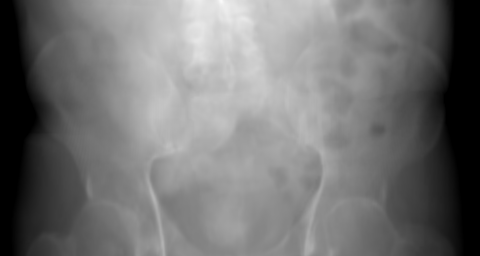
Change from the reference

Reference pose. Each step selects a separately calculated projection.
Synthetic MAISI CT†
Image model and data
MAISI-v2, rectified flow (rflow-ct), generated with 30 inference steps using NV-Generate-CTMR revision 61c4ec709b84. [36]↩
The archived 480 × 256 calculation uses 1,000 incident photons per pixel and an illustrative water-equivalent conversion at 80 keV. Scatter, spectral response and detector noise are absent. This is a simulated radiograph, not a patient acquisition.
The radiographic display maps optical depth from 2 to 5.3 to black–white, with the same window for every pose. Pixels outside that interval saturate only in the display. The difference image shows absolute change in expected counts with a fixed asinh scale, where white is 704.5 counts. It does not show the sign of the change.
Translations use 0.5 mm steps about the reference, and rotations use 0.01 rad steps about the fixed sacral pivot. Playback traverses the recorded poses and reverses at the ends. The time per frame is a display choice.
Pose matrices and display metadata ·Calculation provenance · Original numerical checks
b. Rotation through thirty degrees
Recorded moving pose
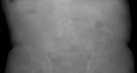
Fixed reference
Reference pose. Thirty-one separately calculated projections span −15° to +15°.
Image model and data
This sweep rotates the object about the centre of the native volume. The source and detector stay fixed. Its pivot and detector field differ from those of the small-motion study above, which rotates about the sacral pivot.
These are simulated primary radiographs of three generated MAISI CT candidates, not patient acquisitions. The full native CT supplies attenuation through the stated water-equivalent approximation at 80 keV. No scatter, spectrum or material-specific calibration is included. AP and PA are cone-beam views and need not be exact horizontal mirrors.
Radiographs use a common optical-depth display interval 0–8. The 480 × 256 detector spans 600 × 480 mm: its pixels have unequal pitches, so the displayed physical aspect is 5:4. No clinical left/right mirror is applied. A/P/R/L/S/I mark body-relative directions.
All 39 distinct projections were checked at 4,096 and 8,192 samples per ray, with three independent reference rays per view. The larger rotation study retains one-degree steps without interpolating between images. Playback timing is illustrative.
Geometry, observations and numerical checks · Source and output digests
3.7 Geometry checks that catch plausible mistakes
A symmetric object can conceal a reflection and two incorrect functions can undo each other’s mistakes (which famously does not make them right). Geometry checks need prescribed coordinates and expected answers that do not come from the same transform chain being checked.
Start with a simple acquisition in millimetres: source at , detector plane at with , and detector axes parallel to world and . A landmark between the source and detector has . Its projected detector coordinates follow by intersecting the line through the source and landmark with the plane:
For , the three labelled landmarks in Table 3.4 give unequal offsets and two magnifications.
| Landmark | World position (mm) | Detector position (mm) |
|---|---|---|
Their labels and asymmetry distinguish a horizontal flip from a vertical flip or an axis exchange. The last point also prevents every landmark from sharing one magnification. Convert these physical detector positions back to continuous pixel coordinates using the same centre and pitch definitions as section 3.3. Rounding to integer pixels would discard part of the check.
Depth controls magnification
- A · depth 500 mm
- B · depth 500 mm
- C · depth 750 mm
Coordinates are in millimetres. The acquisition drawing enlarges transverse dimensions, while the detector plots use equal x and y scales.
Correct projection
A and B magnify by 2, while C magnifies by 4/3.
Horizontal reflection
A and C cross the vertical axis, while B stays on it.
C assigned the wrong depth
Using 500 mm for C gives (−30, 20) mm.
For a separate rotation-centre check, take and a point . A positive quarter-turn about the world direction through must give
Rotating about the world origin instead gives , a different point with a different projection. A transpose error changes the sign of the one-millimetre offset around the correct centre. Table 3.5 extends this check to the other frame and detector conventions.
| Check | Required result | Mistake it exposes |
|---|---|---|
| Identity pose | Points and directions retain their coordinates. | Unexpected offsets or component order. |
| Pure translation | Points shift, while directions remain unchanged. | Translating a direction. |
| Rotation validity | and . | Scale, shear, drift or reflection. |
| Transform then inverse | Recover several asymmetric input points. | Inverse rotation or translation error. |
| Two-step composition | Match independently applying the two transforms in order. | Reversed multiplication. |
| Detector centres | Recover the odd/even centre locations and unequal-pitch example above. | Half-pixel shifts and swapped row/column spacings. |
| Ray endpoints | Recover source and pixel centre at the two parameter bounds. | Wrong origin, direction or segment length. |
| Common rigid frame change | Preserve object-space endpoints and physical lengths. | Inconsistent frame conversion. |
| Prescribed centre rotation | Recover the quarter-turn result above. | Wrong pivot or rotation sign. |
| Local pose derivative | Agree with finite differences using the declared update side. | Wrong frame, sign or lever arm. |
For the final row, choose a six-dimensional direction with translational components in millimetres and rotational components in radians. Use a dimensionless scalar step and, for a left-update check, evaluate the point transform at
As decreases, this approaches the left point-motion expression in section 3.6 with . Check a range of steps through the region where truncation error decreases and before round-off dominates. All three components of the point-displacement comparison are in millimetres, while rotation-matrix residuals are dimensionless. Set their tolerances separately for the chosen arithmetic and coordinate scale.
In our dpt package, these conventions are checked by executable tests in tests/python/test_geometry_contracts.py. The tests exercise the storage and update conventions with explicit points before the projection tests introduce a volume. In particular, a mixed translation-and-rotation increment must exercise the exponential’s translation factor: pure translation and pure rotation can each pass while that coupling is wrong. The package’s later directional checks use the same right composition as Listing 3.2.
The endpoints of the ray we get from this exercise are in the same physical frame as the attenuation field. The next operation is to locate their segment within the volume, map its points to voxel coordinates and integrate along it. That is the task of Chapter 4.
References
- DICOM Standards Committee (2026). DICOM PS3.3 2026c: Information Object Definitions. National Electrical Manufacturers Association. https://dicom.nema.org/medical/dicom/current/output/chtml/part03/PS3.3.html
- Lynch, Kevin M. and Park, Frank C. (2017). Modern Robotics: Mechanics, Planning, and Control. Cambridge University Press. https://doi.org/10.1017/9781316661239