Tracing rays through a sampled volume

A ray can pass through the correct piece of anatomy and still produce the wrong attenuation. Moving its samples by half a voxel changes what it sees near an edge. Using the slice spacing for every direction stretches some paths and shortens others. Both errors can leave a projection looking perfectly respectable, which is inconsiderate of them.

Chapter 3 brought the source and detector into physical object coordinates. We can now ask what attenuation a point on their connecting segment encounters. The volume supplies values at specified locations, and interpolation fills the gaps between them. Integrating that field over physical distance produces the optical depth.

These choices determine the image before GPU execution enters the discussion. They also determine the function we will differentiate in Chapter 5.

We will implement project_optical_depth() by joining three pieces: a physical-to-grid map, a field sampler and a ray integrator. GridSpec supplies the first piece, while the acquisition and pose from Chapter 3 supply the ray. The resulting device array feeds Chapter 2’s transmission operator, completing the path from a stored volume to a primary image.

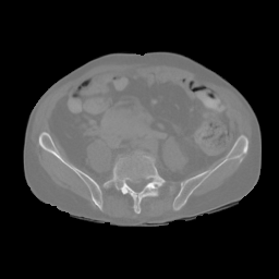
Axial slice

AL

RP

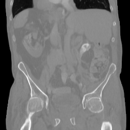
Coronal slice

SL

RI

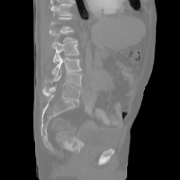
Sagittal slice

SP

AI

AP projection through the whole field

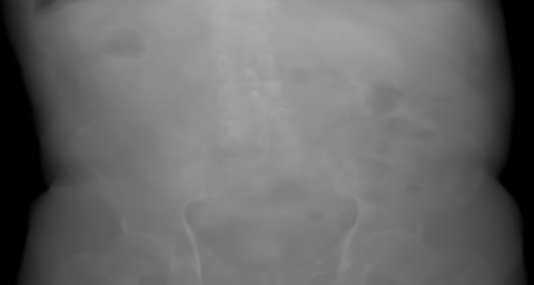
One slice shows one plane of samples. Each projection pixel depends on attenuation along an entire source-to-detector path.

Native grid

256 × 256 × 256 samples

Sample spacing

1.5177865 mm in each direction

Displayed CT interval

−1,000 to +1,000 HU-like values

Attenuation conversion

μ = 0.01837 max(0, 1 + HU/1000) mm⁻¹

Image model and data

These are simulated primary radiographs of three generated MAISI CT candidates, not patient acquisitions. The full native CT supplies attenuation through the stated water-equivalent approximation at 80 keV. No scatter, spectrum or material-specific calibration is included. AP and PA are cone-beam views and need not be exact horizontal mirrors.

Radiographs use a common optical-depth display interval 0–8. The 480 × 256 detector spans 600 × 480 mm: its pixels have unequal pitches, so the displayed physical aspect is 5:4. No clinical left/right mirror is applied. A/P/R/L/S/I mark body-relative directions.

All 39 distinct projections were checked at 4,096 and 8,192 samples per ray, with three independent reference rays per view. The larger rotation study retains one-degree steps without interpolating between images. Playback timing is illustrative.

Geometry, observations and numerical checks · Source and output digests

4.1 What a voxel represents

Fix a photon energy $E$ and suppose the stored values have already been converted to linear attenuation coefficients in $\mathrm{mm}^{-1}$. The energy argument will be suppressed throughout this chapter. A CT intensity or Hounsfield unit needs the material conversion described in Appendix A.11 before it can fill this role.

Let the array have dimensions $N_x,N_y,N_z$, with storage order $A[k,j,i]$. Here $i$ advances along the first grid direction, $j$ along the second and $k$ along the third. These are volume indices, and the detector retains its own column and row indices. Let $\mathbf{o}^O$ be the physical centre of sample $(0,0,0)$, and let the columns of the proper orthogonal matrix $\mathbf{Q}\in\mathrm{SO}(3)$ give the right-handed grid axes in object coordinates. With positive spacings $\Delta_x,\Delta_y,\Delta_z$, define

Equation (4.1) fixes the sample locations independently of array storage. We interpret $A[k,j,i]$ as the attenuation assigned to $\mathbf{x}_{ijk}^O$. A reconstruction may estimate an average over a region rather than a literal point sample. Treating its values as interpolation coefficients is then a modelling choice. We must still declare the locations and the interpolation rule.

A cell associated with an interior sample extends half a spacing in each grid direction. If $\mathbf{u}$ denotes continuous grid coordinates, the union of the stored cells has bounds

The extent in equation (4.2) is $N_a\Delta_a$, while the distance between the first and last sample centres is $(N_a-1)\Delta_a$. Confusing those two lengths moves the boundary by half a voxel at each end. Neither the filename nor the array shape tells us which physical origin a loader has supplied.

A piecewise-constant model assigns each value to its cell. A trilinear model blends neighbouring sample values. Their integrals differ at finite resolution, even with exact integration. Choose the field model before choosing the algorithm that integrates it. Table 4.1 collects the coefficient, grid and support conventions needed to define that field.

4.2 Physical coordinates to array indices

A ray sample arrives as $\mathbf{x}^O$ in millimetres. Subtract the sample origin, rotate into the grid basis and divide by spacing:

Integer grid coordinates select sample centres. Fractional coordinates locate points between them. Apply the spacing division after the basis change: anisotropic scaling and a general rotation do not commute.

For an axis-aligned grid with $\mathbf{o}^O=(10,-20,30)^{\mathsf T}\,\mathrm{mm}$ and spacings $(0.5,0.8,2)\,\mathrm{mm}$, the point $(11,-17.6,34)^{\mathsf T}\,\mathrm{mm}$ maps to $(2,3,2)^{\mathsf T}$. It therefore selects $A[2,3,2]$. The point $(10.25,-19.8,31)^{\mathsf T}\,\mathrm{mm}$ maps to $(0.5,0.25,0.5)^{\mathsf T}$ and needs interpolation. Unequal coordinates and unequal spacings make axis mistakes easier to see.

The coordinate conversion in Figure 4.2 keeps sample centres, cell faces and array indices distinct.

For a contiguous array whose last index varies fastest, the scalar address is

The offset in equation (4.4) counts stored scalars, not millimetres. A strided view needs its actual strides instead. Keeping physical geometry out of the address calculation lets a storage change leave the represented field unchanged.

At the API boundary, establish whether an external origin refers to a first centre or an outer corner. A corner-to-centre conversion adds half a spacing along each grid axis in physical coordinates. Apply that conversion once when constructing the volume geometry. Adding another half voxel in the sampler would translate the entire field.

The origin and basis belong to the volume, even when the array was loaded from a file whose anatomical orientation differs from our object frame. Reordering array axes without updating the map changes the anatomy. Updating both the array and the map consistently changes only its storage description.

Put the grid description in GridSpec and fix it before repeated projection. Its shape is (nz, ny, nx) and spacing is (dx, dy, dz), so the map explicitly connects physical axis order to the x-fastest array. Prepare a contiguous binary32 attenuation field when loading the data, after performing any CT conversion and orientation mapping. The sampler then works with one known representation.

@dataclass(frozen=True, slots=True)
class GridSpec:
    """Oriented anisotropic grid, with origin at the first sample centre.

    Support extends half a sample spacing outside the outer centres. Within
    that support interpolation clamps to the outer sample; beyond it the field
    is zero. Nonzero boundary samples therefore produce a discontinuous field.
    """

    shape: tuple[int, int, int]
    spacing_mm: Vector3
    origin_mm: Vector3 = (0.0, 0.0, 0.0)
    orientation: Matrix3 = IDENTITY

    def __post_init__(self) -> None:
        if len(self.shape) != 3 or any(type(x) is not int or x < 1 for x in self.shape):
            raise ContractError("grid shape is (nz, ny, nx), each a positive integer")
        object.__setattr__(self, "shape", tuple(self.shape))
        object.__setattr__(self, "spacing_mm", vector3(self.spacing_mm, "spacing_mm"))
        object.__setattr__(self, "origin_mm", vector3(self.origin_mm, "origin_mm"))
        object.__setattr__(self, "orientation", rotation_matrix(self.orientation, "orientation"))
        if min(self.spacing_mm) <= 0:
            raise ContractError("grid spacing must be positive")
        if self.voxels > 2**31 - 1:
            raise ContractError("grid exceeds signed 32-bit indexing")

    @property
    def voxels(self) -> int:
        return self.shape[0] * self.shape[1] * self.shape[2]

    def object_to_grid(self, point_mm: Vector3) -> Vector3:
        displacement: Vector3 = cast(
            Vector3, tuple(point_mm[i] - self.origin_mm[i] for i in range(3))
        )
        aligned = matvec(transpose(self.orientation), displacement)
        return cast(Vector3, tuple(aligned[i] / self.spacing_mm[i] for i in range(3)))

    def grid_to_object(self, index: Vector3) -> Vector3:
        scaled: Vector3 = cast(Vector3, tuple(index[i] * self.spacing_mm[i] for i in range(3)))
        aligned = matvec(self.orientation, scaled)
        return cast(Vector3, tuple(aligned[i] + self.origin_mm[i] for i in range(3)))

    @property
    def support(self) -> tuple[Vector3, Vector3]:
        return (-0.5, -0.5, -0.5), (self.shape[2] - 0.5, self.shape[1] - 0.5, self.shape[0] - 0.5)

Choose the support to end at the outer half-cell faces. Interpolate between sample centres, hold the outermost values constant to those faces, and use zero outside. This gives a constant field its full physical box width. A nonzero boundary coefficient creates a jump, which the ray-intersection derivative will have to include.

4.3 Interpolation and the field between samples

The implemented clamped field

Between sample centres, trilinear interpolation blends the nearest two lattice values in each direction. Within an interior interpolation cell, write $\mathbf{m}=\lfloor\mathbf{u}\rfloor$ and $\boldsymbol{\alpha}=\mathbf{u}-\mathbf{m}$. With $w_0(a)=1-a$ and $w_1(a)=a$, the field is

This expression assumes all eight corners lie within the stored array. The weights are nonnegative and sum to one, so a constant interpolation neighbourhood reproduces its constant value. At most eight coefficient reads are needed.

The half-cell extension declared in Listing 4.1 completes the field at the array boundary. First check the physical support in grid coordinates. A point outside it has zero attenuation. Inside it, clamp each coordinate to the range of sample centres before interpolating. At the last centre, use the final valid interpolation interval with weight one at that centre. An axis with only one sample contributes that value without interpolation along the axis. Clamping without the initial support test would extend the edge values indefinitely and turn a finite volume into a surprisingly large object.

The field is continuous between its exterior support faces, but its spatial derivative generally jumps at integer grid planes and clamp transitions. Within an open interpolation cell, the chain rule gives

The physical gradient has units $\mathrm{mm}^{-2}$. The inverse spacing is essential: the same coefficient difference across a thinner interval produces a steeper physical gradient. We will use this derivative when a pose update moves ray samples through the field.

Higher-order interpolation can make the field smoother, but changes its support, reads and approximation properties. Some interpolants can overshoot nonnegative samples. For primary attenuation, a negative interpolated coefficient would imply amplification along that part of the ray. Trilinear interpolation avoids that overshoot for nonnegative inputs through its nonnegative weights.

@wp.func
def sample_field(field: wp.array(dtype=wp.float32), point: wp.vec3d, shape: wp.vec3i) -> Sample:
    """Value and grid-coordinate slope of the half-cell-extended sampled field."""
    result = Sample()
    if not inside_support(point, shape):
        return result
    lower = wp.vec3i()
    fraction = wp.vec3d()
    slope = wp.vec3d()
    for axis in range(3):
        coordinate = wp.clamp(point[axis], wp.float64(0.0), wp.float64(shape[axis] - 1))
        lower[axis] = wp.min(int(wp.floor(coordinate)), wp.max(shape[axis] - 2, 0))
        fraction[axis] = coordinate - wp.float64(lower[axis])
        if point[axis] >= wp.float64(0.0) and point[axis] < wp.float64(shape[axis] - 1):
            slope[axis] = wp.float64(1.0)
    # Separable interpolation reuses the same eight loads for value and slope.
    # Form differences in FP64: FP32 subtraction would lose small field slopes.
    # The compiler removes slope work from the forward-only caller.
    x0, y0, z0 = lower[0], lower[1], lower[2]
    x1 = wp.min(x0 + 1, shape[0] - 1)
    y1 = wp.min(y0 + 1, shape[1] - 1)
    z1 = wp.min(z0 + 1, shape[2] - 1)
    row00 = (z0 * shape[1] + y0) * shape[0]
    row10 = (z0 * shape[1] + y1) * shape[0]
    row01 = (z1 * shape[1] + y0) * shape[0]
    row11 = (z1 * shape[1] + y1) * shape[0]
    v000 = wp.float64(field[row00 + x0])
    v100 = wp.float64(field[row00 + x1])
    v010 = wp.float64(field[row10 + x0])
    v110 = wp.float64(field[row10 + x1])
    v001 = wp.float64(field[row01 + x0])
    v101 = wp.float64(field[row01 + x1])
    v011 = wp.float64(field[row11 + x0])
    v111 = wp.float64(field[row11 + x1])
    dx00, dx10 = v100 - v000, v110 - v010
    dx01, dx11 = v101 - v001, v111 - v011
    fx, fy, fz = fraction[0], fraction[1], fraction[2]
    # Weighted lerp preserves a small endpoint next to a huge neighbour.
    # a+t*(b-a) would erase b at t=1 when the difference rounds to -a.
    ax, ay, az = wp.float64(1.0) - fx, wp.float64(1.0) - fy, wp.float64(1.0) - fz
    x00, x10 = ax * v000 + fx * v100, ax * v010 + fx * v110
    x01, x11 = ax * v001 + fx * v101, ax * v011 + fx * v111
    xy0, xy1 = ay * x00 + fy * x10, ay * x01 + fy * x11
    result.value = az * xy0 + fz * xy1
    # Differentiate corner values before interpolation. Subtracting two
    # already interpolated values can erase a small slope beside a huge
    # orthogonal background, even when its cotangent is representable.
    dx0, dx1 = ay * dx00 + fy * dx10, ay * dx01 + fy * dx11
    dy0 = ax * (v010 - v000) + fx * (v110 - v100)
    dy1 = ax * (v011 - v001) + fx * (v111 - v101)
    dz0 = ax * (v001 - v000) + fx * (v101 - v100)
    dz1 = ax * (v011 - v010) + fx * (v111 - v110)
    result.gradient = wp.vec3d(
        slope[0] * (az * dx0 + fz * dx1),
        slope[1] * (az * dy0 + fz * dy1),
        slope[2] * (ay * dz0 + fy * dz1),
    )
    return result

The value and its grid-coordinate gradient share eight coefficient loads. Each binary32 coefficient is promoted before differences and interpolation are evaluated in binary64. For the value, weighted interpolation retains a small endpoint beside a much larger neighbour. For a slope, the code differences the appropriate corner values before blending them across the other axes. Subtracting two already-interpolated values could erase a small transverse slope beneath a large common background. Those apparently interchangeable algebraic arrangements have different rounding behaviour, so the derivative needs the slope that the stored corner differences still contain.

In the outer half-cell, the field is constant along the clamped axis, so slope suppresses that component. This zero interior slope does not mean moving the support face has zero effect on a ray integral. The clipping calculation below supplies that dependency, and Chapter 5 carries it through the derivative. At a clamp transition or tied interpolation branch, the returned slope is a branch value, not a claim that the field is differentiable there.

Comparison with zero-extended hat interpolation

An alternative treats samples outside the stored index range as zero and interpolates towards them. Define the one-dimensional hat function $\beta$ and, for this comparison, the reference field $\mu_A$ by

Only the nearest two lattice locations in each direction can contribute to equation (4.7), giving at most eight array reads. The local formula in equation (4.5) still applies, but out-of-range coefficients now mean zero. Test index validity before reading them. Clamping an outside index to the nearest stored sample would instead extend the boundary value.

The weights sum to one over the extended lattice. A constant stored region reproduces its constant value wherever all contributing samples have that value. Near the edge of an unpadded array, mixing with the outside zeros creates a ramp. This reference field is continuous, including at its exterior support faces. Its spatial derivative can jump at integer grid planes, and equation (4.6) gives its physical gradient within each open cell.

The ramp fixes the reference support: the field is zero when any grid coordinate lies outside $[-1,N_a]$, and also on the outer faces. This is half a spacing farther out than the cell bounds in equation (4.2). The cell box covers the regions assigned to stored samples, while the interpolation box contains their full hat functions (Figure 4.3). When the intended object has a known zero exterior, an adequate border of zero-valued samples lets us place this interpolation boundary outside the anatomy of interest.

The zero-extended reference and the implemented clamped field therefore differ near the boundary, even when their stored coefficients agree. Section 4.8 checks that difference with a single hat and partial boundary segments. The clipping and quadrature below use the support of whichever field is being integrated.

4.4 Intersecting a ray with the volume

Take the finite object-space segment from Chapter 3, with endpoints $\mathbf{s}^O$ and $\mathbf{q}_p^O$. Its physical length is $d_p=\lVert\mathbf{q}_p^O-\mathbf{s}^O\rVert>0$. Applying the affine grid map to its endpoints gives

The vector $\mathbf{b}_p$ in equation (4.8) is a displacement in grid coordinates. Its Euclidean norm is not a physical ray length when spacing is anisotropic. Keep $d_p$ for integration weights.

For a box with lower and upper bounds $l_a,h_a$ in each grid direction, a nonzero component $b_{p,a}$ gives two plane intersections:

Sorting each pair in equation (4.9) accommodates either ray direction. If $b_{p,a}=0$, the ray is parallel to those planes: it misses the box if $a_{p,a}$ lies outside $[l_a,h_a]$, and otherwise that coordinate imposes no restriction on $t$. Handle this case directly rather than evaluating a division that can produce an infinity or a NaN.

Intersect the three accepted intervals with the source-to-detector segment:

An unconstraining parallel coordinate supplies $(-\infty,+\infty)$ to equation (4.10), or is omitted from the extrema. The interval has positive length only when $t_p^+>t_p^-$. A single tangency contributes zero path length. For the zero-extended hat reference, choose $l_a=-1$ and $h_a=N_a$. The implemented clamped trilinear field and a cellwise-constant volume instead use the half-cell bounds in equation (4.2), but their shared support does not make their interior fields identical.

The clipped physical length is

Equation (4.11) preserves the finite endpoints: a large volume can contain the source or detector, but material beyond either endpoint is still excluded. A miss gives $L_p=0$ and $T_p=1$ immediately, without invoking an interpolation routine on an invalid interval.

Figure 4.4 shows how the slab intervals combine before any attenuation samples are read.

A tiny direction component is not mathematically zero. Replacing every component below a fixed threshold by zero can discard a real, distant intersection. A numerical parallel policy therefore needs a scale-aware error argument and tests against the resulting interval, particularly for long rays and thin volumes.

finite_interval() implements the slab calculation for the library’s half-cell bounds. Initialising its limits to zero and one clips the finite source-to-detector segment before any field samples are requested. A parallel miss produces an empty interval, while an exactly parallel coordinate inside its slab imposes no further restriction. There is no adjustable epsilon that quietly changes a nearly parallel ray into a parallel one.

@wp.func
def finite_interval(origin: wp.vec3d, direction: wp.vec3d, shape: wp.vec3i) -> Interval:
    """Clip a finite segment and retain the active face derivatives.

    Exact parallelism is handled separately; arbitrary epsilon thresholds would
    change the physical interval. At tied faces a derivative is not unique:
    strict comparisons choose the first active axis, a documented branch value.
    """
    interval = Interval()
    interval.lower = wp.float64(0.0)
    interval.upper = wp.float64(1.0)
    for axis in range(3):
        low = wp.float64(-0.5)
        high = wp.float64(shape[axis]) - wp.float64(0.5)
        velocity = direction[axis]
        if velocity == wp.float64(0.0):
            if origin[axis] < low or origin[axis] > high:
                interval.upper = wp.float64(-1.0)
        else:
            first = (low - origin[axis]) / velocity
            last = (high - origin[axis]) / velocity
            if first > last:
                temporary = first
                first = last
                last = temporary
            if first > interval.lower:
                interval.lower = first
                interval.lower_origin_gradient = wp.vec3d(0.0)
                interval.lower_direction_gradient = wp.vec3d(0.0)
                interval.lower_origin_gradient[axis] = -wp.float64(1.0) / velocity
                interval.lower_direction_gradient[axis] = -first / velocity
            if last < interval.upper:
                interval.upper = last
                interval.upper_origin_gradient = wp.vec3d(0.0)
                interval.upper_direction_gradient = wp.vec3d(0.0)
                interval.upper_origin_gradient[axis] = -wp.float64(1.0) / velocity
                interval.upper_direction_gradient[axis] = -last / velocity
    return interval

Keep the selected entry and exit derivatives with the clipped interval. They require only a few per-ray vectors and let the reverse pass follow movement of the bounds. At a tie, strict comparisons choose the first winning axis. This is a deterministic branch convention for a corner where a unique derivative may not exist.

4.5 Quadrature along a physical path

For a nonempty interval, choose a positive integer sample count $M_p$. Equal midpoint samples and their physical weights are

Every weight in equation (4.12) is measured in millimetres, and their sum is $\ell_p$. Midpoints avoid evaluating exactly on the two clipped endpoints. They can still land on internal interpolation knots.

The discrete optical depth is

Equation (4.13) is dimensionless, as the continuous line integral is. Accumulating attenuation values without the distance weights would make a projection depend on the number of samples.

A target physical step $h$ can set $M_p=\max(1,\lceil\ell_p/h\rceil)$. Then the actual step is $\ell_p/M_p\leq h$, so the final sample represents a full equal-width subinterval rather than an accidentally truncated endpoint weight. Another choice fixes $M_p$ during an optimisation stage. The latter keeps the sample-count branch unchanged as pose varies. Chapter 5 will examine the effect of allowing that integer to change.

Midpoint integration is not the only option. For a piecewise-constant field, intersect the ray with the grid planes and accumulate the exact segment lengths through its cells:

The expression in equation (4.14) is exact for that field model, apart from numerical arithmetic. It does not become the exact integral of a trilinear field merely because the cells came from the same array. A trilinear polynomial restricted to an oblique line can be cubic within an interpolation cell, so two-point Gauss integration is exact there if the ray is split at every crossed interpolation plane. That is a different integration strategy again.

Siddon’s method treats the volume as three families of voxel-boundary planes. Their intersections give the exact lengths traversed through piecewise-constant cells, avoiding a separate intersection test for every voxel. [1] We choose trilinear interpolation because it provides within-cell spatial gradients from the stored samples. Midpoint quadrature gives that field a simple streaming implementation, at the cost of integration error. If exact integration of the trilinear field is required, split at its interpolation planes and use the two-point Gauss rule above.

We can measure midpoint error without any volume loader. Along a prescribed physical segment of length $\ell$, let the analytic attenuation be $\mu(s)=\mu_0+b s+c s^2$. Choose coefficients so it is nonnegative on the segment. Its exact optical depth is

Here $b$ has units $\mathrm{mm}^{-2}$ and $c$ has units $\mathrm{mm}^{-3}$. For $M$ equal midpoint intervals, subtracting the sum of squared midpoint locations from equation (4.15) gives

Equation (4.16) predicts both sign and convergence rate of the midpoint error illustrated in Figure 4.5. With $\mu_0=0.01\,\mathrm{mm}^{-1}$, $b=0$, $c=10^{-6}\,\mathrm{mm}^{-3}$ and $\ell=100\,\mathrm{mm}$, the exact optical depth is $4/3$. Counts $M=10,20,40$ give errors $1/1200$, $1/4800$ and $1/19200$.

The forward kernel applies the fixed-count midpoint rule to that clipped interval. One invocation handles one flat detector index: misses write zero, and every intersecting ray uses the prepared samples_per_ray. This makes the discretisation repeatable as pose changes within a clipping branch. It also means physical step size varies with chord length, so choosing a sample count requires convergence checks on the longer relevant paths.

@cache
def get_forward(double_output: bool = False, cell_gauss: bool = False):
    dtype = wp.float64 if double_output else wp.float32

    @wp.kernel(module="unique", module_options=OPTIONS)
    def forward(
        field: wp.array(dtype=wp.float32),
        pose: wp.array(dtype=wp.float64),
        config: Configuration,
        output: wp.array(dtype=dtype),
        status: wp.array(dtype=wp.int32),
    ):
        pixel = wp.tid()
        ray = ray_for_pixel(config, pose, pixel)
        if not valid_ray(ray):
            wp.atomic_or(status, 0, 2)
            output[pixel] = dtype(0.0)
            return
        interval = finite_interval(ray.origin, ray.direction, config.shape)
        integral = wp.float64(0.0)
        if interval.upper > interval.lower:
            if wp.static(cell_gauss):
                traversal = begin_cells(ray, interval, config.shape)
                start = interval.lower
                segments = wp.int64(0)
                limit = (
                    wp.int64(config.shape[0])
                    + wp.int64(config.shape[1])
                    + wp.int64(config.shape[2])
                    + wp.int64(1)
                )
                while start < interval.upper and segments < limit:
                    end = wp.min(traversal.next[0], wp.min(traversal.next[1], traversal.next[2]))
                    if end <= start:
                        wp.atomic_or(status, 0, 2)
                        break
                    radius = (end - start) * wp.float64(0.5)
                    centre = start + radius
                    offset = radius / wp.sqrt(wp.float64(3.0))
                    for node in range(2):
                        position = centre + wp.float64(2 * node - 1) * offset
                        integral += (
                            radius
                            * sample_field(
                                field, ray.origin + position * ray.direction, config.shape
                            ).value
                        )
                    start = end
                    traversal = advance_cells(traversal, ray, config.shape, end, interval.upper)
                    segments += wp.int64(1)
                if start < interval.upper:
                    wp.atomic_or(status, 0, 2)
                integral *= ray.length
            else:
                step = (interval.upper - interval.lower) / wp.float64(config.samples)
                for sample in range(config.samples):
                    position = interval.lower + (wp.float64(sample) + wp.float64(0.5)) * step
                    point = ray.origin + position * ray.direction
                    if not finite_point(point):
                        wp.atomic_or(status, 0, 2)
                    integral += sample_field(field, point, config.shape).value
                integral *= ray.length * step
        output[pixel] = dtype(integral)
        if not wp.isfinite(output[pixel]):
            wp.atomic_or(status, 0, 2)

    return forward

ray.length remains a millimetre distance even though ray.origin and ray.direction use grid coordinates. Multiplying it by step supplies the physical quadrature weight. Sample values accumulate in a binary64 register. The default output is rounded to binary32; precision="float64" retains the binary64 result while leaving the stored field coefficients unchanged. No positions or interpolation weights are written to a ray-by-sample array. The status flag records invalid coordinates or an unrepresentable output, and a zero written on a failed ray is not permission to interpret the result as vacuum.

The alternative integration="cell_gauss" follows that cell-split rule. It costs extra plane intersections but removes the quadrature error within each trilinear piece. Use it when midpoint refinement is too expensive or when moving midpoint samples create troublesome gradient jumps. Chapter 11 uses it for the completed pose fit.

4.6 A GPU projection operator

Let us assign each detector ray to one CUDA thread. Each thread clips its ray to the volume, accumulates optical depth in registers and writes the result to its detector pixel. All threads read from the same volume without modifying it. Neighbouring threads write adjacent output values, but their rays may cross the volume obliquely, so adjacent writes do not imply contiguous reads.

Write a Warp kernel over the flat pixel index, using wp.tid() to identify the ray. Allocate the field and geometry before repeated launches, and form each sample position from its index inside the loop. This keeps the volume on the GPU and avoids a tensor containing every point along every ray. The Warp programming guide describes the kernel and array model used here.

For fixed geometry and quadrature, the complete operator is linear in the stored coefficients. Flattening them into $\mathbf{a}$ gives

where $B_v$ is the tensor-product basis from equation (4.7) for the zero-extended reference. For the implemented field, use the corresponding clamped interpolation weights inside its half-cell support. Both choices remain linear in the stored coefficients. The matrix in equation (4.17) describes the selected operator, but we need not store it. Evaluating its nonzero contributions while traversing each ray avoids a potentially enormous sparse matrix and keeps the interpolation convention visible in the calculation. The interface in Table 4.2 makes the required geometry, coefficient storage and repeated-call behaviour explicit.

Each thread writes to a distinct detector pixel, so the forward projection needs no atomic operations. It still sums contributions along each ray, and the precision of that sum must be chosen independently of the volume’s storage precision. Tests for long rays should include many small contributions added after larger ones, when rounding can erase their effect. If optical depth is not needed separately, evaluating the exponential in the projection kernel can avoid a second kernel launch and a read of the intermediate optical-depth image. Retaining optical depth as an explicit output, however, supports log-domain objectives and diagnostics.

Keep optical depth as the explicit output of project_optical_depth(). prepare_projection() binds the grid, detector, quadrature and CUDA stream, then allocates reusable workspace. The caller supplies the field, packed pose and output array. Separating preparation from evaluation avoids device allocation during a pose search.

def project_optical_depth(
    mu: Any,
    pose: Any,
    *,
    workspace: ProjectionWorkspace,
    out_L: Any,
    stream: Any = None,
    tape: Any = None,
    validate: bool = True,
) -> None:
    """Overwrite dimensionless optical depth for every finite detector ray.

    mu is a flat non-negative FP32 field in inverse mm. pose is twelve FP64
    values (R_WO row-major, t_WO in mm). out_L is flat row-major detector
    storage in the precision declared by ProjectionSpec. A checked call
    synchronises domain diagnostics before writing and
    range diagnostics afterwards. Unchecked calls promise valid current inputs
    and require check_status() at the next acceptance checkpoint.
    """
    ensure_tape(tape)
    _inputs(mu, pose, workspace, stream)
    if workspace._recorded_tape is not None:
        raise ContractError("finish or discard the outstanding projection tape before reuse")
    ctx = workspace.context
    ctx.array(out_L, "out_L", dtype=workspace.dtype, shape=(workspace.geometry.pixels,))
    ctx.disjoint([("mu", mu), ("pose", pose)], [("out_L", out_L)])
    if tape is not None:
        _check_tape_arrays(mu, pose, out_L, workspace)
    if validate:
        _validate(mu, pose, workspace)
    ctx.wp.launch(
        workspace._kernels.get_forward(
            workspace.spec.precision == "float64", workspace.spec.integration == "cell_gauss"
        ),
        dim=workspace.geometry.pixels,
        inputs=[mu, pose, workspace._configuration],
        outputs=[out_L, workspace._status],
        stream=workspace.stream,
        block_dim=_BLOCK,
        record_tape=False,
    )
    if validate:
        workspace.check_status()
    if tape is not None:
        _record(tape, mu, pose, out_L, workspace)

Check input values and buffer compatibility before the first projection, including overlaps that could overwrite the field or pose. Reused fixed data need not be rescanned at every iteration, but each trial pose must remain valid. The kernel’s numerical status must be checked before its output is accepted.

The validate=False option lets an enclosing solver take responsibility for those checks. It omits the value scan, not the physical or storage requirements.

The next call passes out_L to transmit() on the same stream, with independently prepared output destinations. Keeping the two operators separate gives both counts and log transmission access to the same optical depths. It also lets the reverse chain reuse their independently tested numerical policies.

A variable-step projector can give neighbouring rays different loop lengths. Our fixed-count kernel removes that source of divergence for intersecting rays, although misses exit early and interpolation branches can differ. Measure the remaining divergence together with memory throughput and occupancy. A block cooperating on one long ray may expose more parallelism but introduces a reduction, changes rounding order and spends more threads on short rays. The useful choice depends on the detector size, path-length distribution and device.

A trilinear sample requests at most eight coefficients. Cache reuse can reduce the associated memory transactions, while scattered access can make each requested scalar expensive. Profile register pressure, achieved occupancy and cache behaviour on the actual acquisition. The launch configuration should follow those measurements rather than a generic claim that one block size is best.

4.7 Resolution, truncation and convergence

There are three different approximations we need to keep apart.

• Field approximation. Sampling the anatomy and choosing an interpolant produces a field $\mu_A$. The sample spacing, coefficient values and boundary extension determine what this field can represent. Fine structures may be lost or blurred before any ray is integrated; taking more samples along that ray cannot restore them.
• Quadrature error. Numerical quadrature replaces the exact line integral of $\mu_A$ with a finite weighted sum. Its error depends on the integration rule, sample placement and variation of the field along the ray, including crossings of interpolation knots. Refining the quadrature tests how accurately we integrate the chosen field, not how faithfully that field represents the anatomy.
• Floating-point error. Finite-precision coordinate calculations, interpolation, weighting and accumulation perturb the exact-arithmetic quadrature. Small contributions can disappear when added to a much larger running total, and rounding the final output introduces another error. Increasing the sample count does not guarantee that this error decreases; arithmetic precision and evaluation order need their own checks.

If $L$ denotes the intended continuous-field integral, $L_A$ its exact interpolated-field counterpart and $\widehat L$ the exact-arithmetic quadrature, then

Equation (4.18) tells us what a convergence experiment can establish. Halving the integration step while keeping the array fixed tests quadrature convergence towards $L_A$. It cannot recover anatomy that the array and interpolation have already lost.

Use two references to separate these errors. First integrate a prescribed continuous field analytically. Then integrate the actual sampled interpolant exactly within each crossed piece, using the two-point Gauss rule. The second reference must use the uploaded coefficients, including their storage rounding. This isolates quadrature error from the approximation already introduced by sampling the field.

Compare midpoint refinements with the sampled-field reference, and grid refinements with the continuous field. A positive quadratic field in a fixed box supplies a convenient continuous reference.

A grid-refinement study holds the physical object and acquisition fixed, samples the same analytic field on successively finer grids and reduces quadrature error enough to expose the field approximation. Keep the zero boundary outside the prescribed object’s support at every resolution. Changing array dimensions while retaining the old spacing changes the physical object size, which is a different experiment.

The boundary extension also makes truncation a physical modelling question. If tissue reaches an edge of the supplied array, the hat reference ramps towards zero while the implemented field holds the edge value to a half-cell face and then drops to zero. Refining quadrature integrates the chosen exterior more accurately. It does not tell us what attenuation was outside the scan. Padding with known zeros is appropriate where the exterior is actually known to be zero, and it is not a reconstruction of missing tissue.

Errors in optical depth pass nonlinearly into transmission. For a perturbation $\delta L$,

For small errors, equation (4.19) gives a relative transmission error of approximately $-\delta L$. A heavily attenuated ray can have a tiny absolute count error while retaining a substantial relative transmission error. Report optical-depth error alongside the quantity the application actually compares.

For smooth fields and a suitable uniform midpoint sequence, a quadratic error regime is expected. An unsplit interpolation knot interrupts the smoothness assumptions behind the usual second-derivative error formula. A finite study may also reach a plateau where field error or floating-point error dominates. The slope of one log-log plot is therefore useful only with the field, quadrature and arithmetic held to a declared comparison.

4.8 Boundary and consistency checks

We begin with coordinates whose answers fit on a page.

• An axis-aligned box gives a known chord length.
• A ray that misses it has zero optical depth.
• Reversing the endpoints leaves the integral unchanged, provided the field and physical segment are unchanged.

These tests detect mistakes that an anatomical projection can conceal.

The zero-extended hat reference also has a compact exact check. Put one nonzero coefficient $a$ at grid index $(0,0,0)$ and all other coefficients at zero. Trace a grid-axis ray through that sample, with its other two grid coordinates fixed at zero and endpoints beyond the full support. Then

The triangular area in equation (4.20) tests the zero extension and its physical width together. For a single-sample axis, $N_x=1$, clipping to both half-cell faces retains only three quarters of that area. With $N_x\geq2$, the boundary sample loses only its outer eighth, so clipping retains seven eighths. A clamped extension has a different support again. These are distinguishable numerical models, not interchangeable boundary conveniences.

For the implemented field, use a constant box to test the full half-cell chord and use an outer-sample case to test the clamp. A single nonzero boundary sample beside a zero neighbour contributes a constant half-cell followed by a linear decline to the next centre. The resulting area can happen to match the complete hat area even though the functions differ. Shorten the segment to the outer half-cell and the two values separate. Tests need such partial segments: one agreeing total integral is insufficient to identify the boundary model.

For nonnegative coefficients and quadrature weights, the discrete operator has useful ordering properties:

The transmission inequality in equation (4.21) concerns finite real optical depths, and stored transmission may underflow to zero. The two optical-depth inequalities are direct tests of interpolation and accumulation signs. A negative result from finite nonnegative inputs cannot be explained by a different physical interpretation of primary attenuation. The independent cases in Table 4.3 separate these sign errors from geometry and quadrature errors.

Set absolute and relative error tolerances in the quantity being tested. Coordinates are in millimetres, while optical depth is dimensionless. Near zero, an absolute optical-depth tolerance carries the comparison, because a relative error alone divides by a vanishing reference. Keep a separate tolerance for the quadrature error predicted by an analytic test and the floating-point difference between two evaluations of the same quadrature.

Connect project_optical_depth() to transmit() and render the same volume at two nearby poses. The changed image now follows from explicit coordinate maps, a chosen interpolant and physical distance weights. Chapter 5 will carry derivatives through this construction, including the moving clipped interval.

References

- Siddon, Robert L. (1985). Fast calculation of the exact radiological path for a three-dimensional CT array. Medical Physics, 12(2), 252-255. https://doi.org/10.1118/1.595715