Reconstructing a volume from its X-ray projections
Here the unknown is the attenuation field itself. We use projection gradients to recover it, with regularisation to constrain what the available views leave uncertain.
The registration problem gave us a volume and asked where it was. Reconstruction takes away the volume. We keep the calibrated source and detector positions, supply several radiographs, and estimate the attenuation field that could have produced them. The forward calculation is familiar, but the unknown now has one coefficient per voxel, which rather changes the storage bill.
Chapter 4 defined the sampled field and Chapter 5 its discrete derivatives. We will use those operators directly, first with a primary monochromatic count model. Chapter 8’s spectral model then lets us ask a harder question: which material mixtures are consistent with energy-resolved measurements?
The scalar example implements fixed-geometry voxel reconstruction with a quadratic spatial penalty. The complete material workflow in §12.8 extends that calculation to an assigned water/bone field from CT-derived anatomy, with simulated spectral observations and independent recovery checks. Its assigned fractions are not measurements of patient composition.
12.1 Specify the unknown volume and measured projections
Let contain nonnegative attenuation coefficients in . They are the samples of the trilinearly interpolated field from Chapter 4. The grid shape is , x varies fastest in memory, and its origin is the first sample centre. Spacing is specified along the grid’s x, y and z axes. An orientation matrix places those axes in object coordinates, and a fixed object-to-world transform places the volume in the calibrated acquisition.
For view , write the predicted optical depths as
includes ray intersections with the volume support, the chosen midpoint quadrature and interpolation weights. Its entries have units of millimetres. contains the calibrated expected open-beam counts, and is the predicted mean count image. The observed integer counts are . Conditioning on the supplied open-beam calibration treats its uncertainty as negligible. A noisy flat-field estimate would require another part of the statistical model.
This model assumes independent photon counts, primary transmission and a monochromatic beam or an effective-energy approximation justified for the acquisition. An energy-integrating detector’s processed pixel values do not become Poisson counts because we rename the file. Scatter, electronic noise and spectral hardening can all produce structured discrepancies that the optimiser will otherwise try to explain with incorrect attenuation.
The example requires an initial attenuation volume as supplied input, together with measured counts and open-beam means for every view. It neither interprets Hounsfield units nor derives an attenuation conversion from a material name. All source arrays carry units, checksums and provenance. Before using or redistributing acquired scans and independent reference volumes, document the rights governing those uses.
Figure 12.1 separates known geometry from unknown coefficients. A coefficient whose interpolation support misses every measured ray has a zero column in the combined projector. No choice of optimiser can make those measurements constrain it.
Four measured rays in a grid section
Unit grid spacing. Hatching includes the corner basis’s half-cell boundary extension.
The ray operator maps coefficients to optical depth.
Its full basis support misses the rays, hence every quadrature sample on them.
For changes preserving nonnegativity, these measurements give no preference. Additional rays or a prior supply different information.
12.2 Derive the discrete volume gradient
For the fixed acquisition, is linear in the voxel coefficients. The exponential that follows it is nonlinear. A detector-space objective supplies a cotangent , giving
We use ordinary Euclidean inner products on the stored coefficient and detector vectors. Consequently, is the matrix transpose of the implemented discrete map. A continuous backprojection formula, or the transpose of a different interpolation rule, need not give this derivative. If we instead defined volume and detector inner products through mass matrices and , their weighted adjoint would be . Those weights cannot be added twice, once in the objective and again as an unexplained voxel-volume factor.
Each reverse ray revisits its quadrature samples and scatters the seed through the same interpolation weights. Support clipping and the constant extension between the outer sample centres and half-cell faces remain the forward operator’s rules. Siddon’s radiological-path calculation is a useful reference for a different, cellwise-constant discretisation, but using its traversal does not make it the exact transpose of our sampled trilinear field. [1]
The implementation sets active_volume=True and active_pose=False. It clears the shared voxel gradient once, then accumulates each view’s contribution with projection_vjp. No system matrix or ray-by-sample tape is stored. The listing includes the count-space chain, so its seed differentiates the same objective and passes through the existing FP32 cotangent interfaces.
    def evaluate(self, volume: Any, volume_wp: Any, *, gradient: bool) -> float:
        """Evaluate every supplied view before an update; add the prior once."""
        if gradient:
            self.gradient.zero_()
        loss = 0.0
        for view in self.views:
            project_optical_depth(
                volume_wp,
                self.pose,
                workspace=view["projection"],
                out_L=view["depth"],
                stream=self.stream,
            )
            transmit(
                view["depth"],
                view["beam"],
                workspace=view["transmission"],
                out_counts=view["prediction"],
                stream=self.stream,
            )
            evaluate_objective(
                view["prediction"],
                view["observed"],
                workspace=view["objective"],
                out_loss=view["loss"],
                out_seed=view["image_seed"] if gradient else None,
                stream=self.stream,
            )
            if gradient:
                transmission_vjp(
                    view["depth"],
                    view["beam"],
                    seed_counts=view["image_seed"],
                    workspace=view["transmission"],
                    out_grad_L=view["depth_seed"],
                    stream=self.stream,
                )
                projection_vjp(
                    volume_wp,
                    self.pose,
                    adj_L=view["depth_seed"],
                    workspace=view["projection"],
                    out_mu=self.gradient_wp,
                    accumulate=True,
                    stream=self.stream,
                )
            loss += float(view["loss"].numpy()[0])
        loss += self.regularise(volume, gradient=gradient)
        if not math.isfinite(loss):
            raise NumericalError("The objective is non-finite; inspect counts and model range.")
        if gradient and not bool(self.torch.isfinite(self.gradient).all().item()):
            raise NumericalError("The volume gradient overflowed; discard this evaluation.")
return lossFigure 12.2 follows these quantities through both directions. Before accepting numerical results, test with independently chosen vectors and check the composed objective along volume perturbations. A reverse pass that merely returns finite numbers has met a rather modest ambition.
Forward · one calibrated view k
- Voxel coefficients
Unknown attenuation, with fixed grid and geometry.
- Optical depth
Ray quadrature and interpolation are inside Aₖ.
- Mean counts
The open-beam calibration is fixed.
- View loss
Compare with that view’s observed counts.
Reverse · from the loss to the volume
- Seed the scalar loss
One view’s contribution to the summed objective.
- Count seed
Differentiate the selected measurement objective.
- Optical-depth seed
Pull the seed through the exponential.
- Volume contribution
Use the same discrete weights in reverse.
Ordinary Euclidean inner products on stored arrays define the transpose. No extra voxel-volume factor belongs in this data term.
For positive predicted means:
Count-seed arithmetic
The algebraic form of the optical-depth seed does not remove the count-seed interface’s numerical range limits.
12.3 Choose the likelihood and regularisation
For independent Poisson observations, the code minimises the half-deviance, which differs from the negative log-likelihood by an observation-only constant:
For , the contribution is , and we never evaluate as an intermediate observation term. For positive , the mean must be positive. The count derivative is , so the algebraically composed optical-depth derivative simplifies to . Thus
Under these fixed-geometry primary-count assumptions, the likelihood is convex in attenuation. That does not guarantee strict convexity or uniqueness. A null space survives wherever different coefficient fields have identical measured projections. Spectral mixing and joint geometry estimation will not generally retain this convenient structure.
The application composes the existing objective and transmission VJPs. They store count seeds in FP32, so an intermediate can exceed their range even when the simplified depth derivative is representable. Checked calls reject that evaluation. They also reject a mean rounded to zero beside a positive observation. The example does not silently floor it.
Any voxel change in the likelihood’s null space is invisible to the measurements. A spatial penalty states which possible fields we prefer. Here we favour smaller differences between neighbouring coefficients, using quadratic neighbouring-voxel regularisation:
contains each neighbouring pair along axis once, is that axis’s spacing and . Edges beyond the grid are omitted. This adds no boundary penalty against exterior zero, even though the projector’s field is zero outside its support. has units of , so has units of millimetres when the count objective is dimensionless. Replacing millimetres with centimetres therefore changes the numerical regularisation coefficient as well as the grid metadata.
For one edge, the regulariser adds to voxel and its negative to voxel . The implementation uses FP64 differences and loss reductions, with FP32 updates to the stored volume gradient.
    def regularise(self, volume: Any, *, gradient: bool) -> float:
        """Quadratic physical-space differences; omit edges beyond the grid."""
        self.volume64.copy_(volume)
        penalty = 0.0
        for low, high, grad_low, grad_high, scratch, coefficient in self.edges:
            difference, derivative = scratch
            self.torch.sub(high, low, out=difference)
            if gradient:
                # Scale in FP64 before the FP32 accumulation boundary.
                difference.mul_(coefficient)
                derivative.copy_(difference)
                grad_low.sub_(derivative)
                grad_high.add_(derivative)
                # Restore unscaled differences for the objective.
                self.torch.sub(high, low, out=difference)
            difference.square_()
            self.torch.sum(difference, dim=(0, 1, 2), out=self.scalar)
            penalty += 0.5 * coefficient * float(self.scalar.item())
return penaltyQuadratic smoothing penalises sharp genuine boundaries alongside noise. Total variation or a learned prior would change that bias and require a different solver or derivative. Here, nonnegativity is enforced by projection after an update. Unlike an exponential parameterisation, projection permits exact zero attenuation without driving a latent variable towards minus infinity.
The driver uses summed likelihood terms and all supplied pixels. Saturated or missing observations need an explicitly extended masking or censoring model before use, while zero observed counts are valid measurements. Choose and stopping rules on separate development data or a predefined protocol, keeping the final evaluation volume out of those choices.
12.4 Plan the GPU reconstruction iteration
The volume, trial volume, voxel gradient and update displacement remain on CUDA. Per-view observations, means and derivative buffers also stay there. Torch owns the voxel arrays, and Warp receives zero-copy views of their storage, and both frameworks use the same CUDA stream. Ownership lasts through the final stream synchronisation, including exception paths. The Warp interoperability documentation describes the array and stream conversions used here.
An iteration evaluates every supplied view at the accepted volume, adds regularisation once, and chooses a projected step. With ,
The line search accepts strict decrease satisfying , for configured . It reduces geometrically when this condition fails. The gradient has units of millimetres, so has units of . The stopping quantity is at a fixed configured reference step, measured in millimetres. A small objective change alone does not establish constrained stationarity.
    def solve(
        self, callback: Callable[[int, dict[str, Any]], None] | None = None
    ) -> dict[str, Any]:
        """Solve with optional observation of accepted updates only.

        The callback receives the stable one-based accepted iteration and a
        detached history dictionary after ``mu`` has been updated. It may read
        or export the accepted fields but must not mutate solver state. Callback
        exceptions propagate with the last accepted volume intact.

        An optional fixed mapping step separates the stationarity diagnostic
        from the initial Armijo trial. Omitting it preserves the original
        diagnostic at ``initial_step_mm_inverse_squared``.
        """
        policy = self.policy
        mapping_step = (
            policy.initial_step_mm_inverse_squared
            if policy.mapping_step_mm_inverse_squared is None
            else policy.mapping_step_mm_inverse_squared
        )
        history: list[dict[str, Any]] = []
        reason = "iteration_budget"
        for iteration in range(policy.iterations):
            loss = self.evaluate(self.mu, self.mu_wp, gradient=True)
            step = policy.initial_step_mm_inverse_squared
            mapping, _ = self.displacement(mapping_step)
            if not math.isfinite(mapping):
                raise NumericalError("The trial update overflowed; reduce the initial step.")
            if mapping <= policy.gradient_mapping_tolerance_mm:
                reason = "projected_gradient_tolerance"
                break
            accepted = False
            for attempt in range(policy.maximum_backtracks):
                if step == 0:
                    break
                _, slope = self.displacement(step)
                if not math.isfinite(slope) or slope >= 0:
                    step *= policy.backtracking_factor
                    continue
                # Trial value evaluation leaves the accepted gradient unchanged.
                # Domain/range errors abort with the last accepted volume intact.
                trial_loss = self.evaluate(self.trial, self.trial_wp, gradient=False)
                if trial_loss < loss and trial_loss <= loss + policy.armijo * slope:
                    self.mu.copy_(self.trial)
                    history.append(
                        {
                            "iteration": iteration + 1,
                            "loss_before": loss,
                            "loss_after": trial_loss,
                            "step_mm_inverse_squared": step,
                            "backtracks": attempt,
                            "mapping_mm_before": mapping,
                        }
                    )
                    accepted = True
                    if callback is not None:
                        callback(iteration + 1, dict(history[-1]))
                    break
                step *= policy.backtracking_factor
            if not accepted:
                reason = "line_search_failed"
                break
        # Trial buffers may describe a rejected volume; refresh accepted outputs.
        final_loss = self.evaluate(self.mu, self.mu_wp, gradient=True)
        final_mapping, _ = self.displacement(mapping_step)
        if final_mapping <= policy.gradient_mapping_tolerance_mm:
            reason = "projected_gradient_tolerance"
        return {
            "termination": reason,
            "accepted_steps": len(history),
            "final_objective": final_loss,
            "final_gradient_mapping_mm": final_mapping,
            "history": history,
}Failed searches and iteration budgets are recorded separately from the projected-gradient criterion. Trial evaluations leave the accepted gradient intact. The final projection refresh matters: the most recently rendered trial may have been rejected.
The prepared volume workspace contains five FP32 arrays and two FP64 arrays, or bytes before scalar buffers, plus six FP32 detector arrays per view and the canonical operator scratch. There is no optimiser history proportional to the iteration count. Torch finite checks and scalar reductions can allocate temporary storage. Checked operator calls synchronise, and Python receives scalar losses and line-search decisions.
All views are retained on device in this implementation. When all views do not fit, processing bounded groups requires accumulating the full gradient before each update. Updating after each group would instead change the optimisation schedule. Profiling must distinguish the projector’s memory access and FP32 atomic contention from the additional reduction and synchronisation costs. Atomic accumulation does not promise identical bits between runs, even though the objective contains no randomly sampled views.
12.5 Reconstruct with fewer or restricted views
Sparse angular sampling leaves gaps between otherwise broadly distributed views. Limited-angle acquisition restricts the directions themselves. Both can produce an apparently stable minimiser, but they constrain different structures poorly. Adding more views inside a narrow angular interval does not supply the missing directions outside it.
Direct optimisation of voxel fields is also used by DiffVox, which combines differentiable rendering with its own reconstruction formulation. This lets us study voxel reconstruction before introducing a neural field. [37] A flexible representation can express more possible volumes, but it cannot establish which unmeasured detail is correct.
Why the earlier sparse-versus-dense comparison needs matched stopping states
Figure 12.3 compares 144 broadly distributed views with 36 broad or 36 limited-angle views, holding the inverse grid and field of view fixed for each anatomy. The broad arrangements cover a full orbit, while the limited arrangement spans −60° to 60°. Three tilts are used in each arrangement. All three receive 28.8 million expected incident photons per detector pixel over the fitting acquisition: 200,000 per view in the dense case and 800,000 in the others. This fixes incident photon number without claiming equal absorbed dose. Another 24 whole views are reserved for evaluation, including nine inside the limited yaw interval and fifteen outside it.
For the monochromatic observations, the baseline is post-log penalised weighted least squares, using the same counts, geometry, starting field and physical penalty as Poisson reconstruction. Its fixed observed-count weights approximate the inverse log-data variance, and zero counts are excluded and reported. Both use the same projector, so this compares objectives rather than independently implemented forward models. The spectral comparison instead uses separately simulated three-channel observations. Its two methods differ in their projected optimisation step: one uses a fixed material metric and the other uses a Euclidean projection. The latter was prescribed for dense coverage only. Filtered backprojection cannot simply be transferred from parallel-beam to this cone-beam geometry without changing the algorithm.
The forty fits cover two anatomies and two noise replicates. Every fit reached its prescribed time limit with stationarity still unmet. The dense fits had 600 seconds each, and the sparse and limited fits had 300 seconds each. In all four matched anatomy/replicate pairs, the sparse material-metric fit has lower whole-box bone-fraction RMSE than its dense counterpart. It also completed 135–191 accepted updates against 70 for the dense fits. These records show the interaction between acquisition and the cost of an iteration. They cannot isolate the effect of angular sampling or rank converged solutions. The figure retains every outcome and uses the same physical planes and display windows throughout.
The retained checkpoints show why the stopping point matters. At 50 accepted updates, the case-2 dense fits have slightly lower bone-fraction RMSE than the sparse fits, about 0.106 against 0.109; sparse overtakes them by the unequal final stopping points. Case 0 already slightly favours sparse at 50 updates. Optimisation progress therefore contributes to the recorded comparison, but does not explain every difference. Matching updates would still leave different acquisitions and objective geometries, so it would not by itself rank converged reconstructions either.
Scalar Poisson
An attenuation field from separately simulated monochromatic 80 keV counts.
Scalar attenuation at 80 keV · Axial (z = 0 mm)
Assigned reference

Broad dense

144 views · 47 accepted updates
Broad sparse

36 views · 92 accepted updates
Limited angle

36 views · 92 accepted updates
Axial (z = 0 mm). Black → white: 0 to 0.05 mm⁻¹. Matched physical extent and display window.
Signed errors and display clipping
Broad dense: recovered − reference

Blue -0.01 · pale 0 · red 0.01 mm⁻¹
Broad sparse: recovered − reference

Blue -0.01 · pale 0 · red 0.01 mm⁻¹
Limited angle: recovered − reference

Blue -0.01 · pale 0 · red 0.01 mm⁻¹
Reference slice: 0 pixels below the window and 0 above.
- Broad dense: recovered slice 0 below and 0 above. Signed error 0 below and 0 above.
- Broad sparse: recovered slice 0 below and 0 above. Signed error 0 below and 0 above.
- Limited angle: recovered slice 0 below and 0 above. Signed error 0 below and 0 above.
Clipping affects displayed pixels. Numerical errors use the complete recorded fields.
Scalar attenuation at 80 keV · Coronal (y = 0 mm)
Assigned reference

Broad dense

144 views · 47 accepted updates
Broad sparse

36 views · 92 accepted updates
Limited angle

36 views · 92 accepted updates
Coronal (y = 0 mm). Black → white: 0 to 0.05 mm⁻¹. Matched physical extent and display window.
Signed errors and display clipping
Broad dense: recovered − reference

Blue -0.01 · pale 0 · red 0.01 mm⁻¹
Broad sparse: recovered − reference

Blue -0.01 · pale 0 · red 0.01 mm⁻¹
Limited angle: recovered − reference

Blue -0.01 · pale 0 · red 0.01 mm⁻¹
Reference slice: 0 pixels below the window and 0 above.
- Broad dense: recovered slice 0 below and 0 above. Signed error 0 below and 0 above.
- Broad sparse: recovered slice 0 below and 0 above. Signed error 0 below and 2 above.
- Limited angle: recovered slice 0 below and 0 above. Signed error 0 below and 0 above.
Clipping affects displayed pixels. Numerical errors use the complete recorded fields.
Scalar attenuation at 80 keV · Sagittal (x = 0 mm)
Assigned reference

Broad dense

144 views · 47 accepted updates
Broad sparse

36 views · 92 accepted updates
Limited angle

36 views · 92 accepted updates
Sagittal (x = 0 mm). Black → white: 0 to 0.05 mm⁻¹. Matched physical extent and display window.
Signed errors and display clipping
Broad dense: recovered − reference

Blue -0.01 · pale 0 · red 0.01 mm⁻¹
Broad sparse: recovered − reference

Blue -0.01 · pale 0 · red 0.01 mm⁻¹
Limited angle: recovered − reference

Blue -0.01 · pale 0 · red 0.01 mm⁻¹
Reference slice: 0 pixels below the window and 0 above.
- Broad dense: recovered slice 0 below and 0 above. Signed error 0 below and 0 above.
- Broad sparse: recovered slice 0 below and 0 above. Signed error 0 below and 0 above.
- Limited angle: recovered slice 0 below and 0 above. Signed error 0 below and 1 above.
Clipping affects displayed pixels. Numerical errors use the complete recorded fields.
First whole withheld view · 80 keV monochromatic channel
Simulated observation

Broad dense: prediction

Broad sparse: prediction

Limited angle: prediction

Common negative-log window 0 to 8. This entire view was withheld from every fit.
Withheld-view residuals and display clipping
Broad dense: observation − prediction

Blue -5 · pale 0 · red 5 predicted Poisson standard deviations.
548 pixels below the residual window and 371 above.
Prediction display: 0 below and 0 above.
Broad sparse: observation − prediction

Blue -5 · pale 0 · red 5 predicted Poisson standard deviations.
295 pixels below the residual window and 329 above.
Prediction display: 0 below and 0 above.
Limited angle: observation − prediction

Blue -5 · pale 0 · red 5 predicted Poisson standard deviations.
193 pixels below the residual window and 184 above.
Prediction display: 0 below and 0 above.
Observation display: 2098 pixels below the window and 0 above.
The residual divides observation minus prediction by the square root of the predicted count. Its scale is fixed before evaluation.
Acquisition angles and stopping conditions
Broad dense
144 views × 200,000 expected incident photons per detector pixel per view.
Time limit. Stationarity criterion unmet. Recorded solve: 609.19 s.
Broad sparse
36 views × 800,000 expected incident photons per detector pixel per view.
Time limit. Stationarity criterion unmet. Recorded solve: 302.89 s.
Limited angle
36 views × 800,000 expected incident photons per detector pixel per view.
Time limit. Stationarity criterion unmet. Recorded solve: 302.92 s.
Rows show tilt and dots show the recorded yaw angles. Equal incident photon population does not imply equal patient dose or equivalent scalar and spectral measurements.
Scalar log-WLS
An attenuation field from separately simulated monochromatic 80 keV counts.
Scalar attenuation at 80 keV · Axial (z = 0 mm)
Assigned reference
Broad dense

144 views · 60 accepted updates
Broad sparse

36 views · 117 accepted updates
Limited angle

36 views · 117 accepted updates
Axial (z = 0 mm). Black → white: 0 to 0.05 mm⁻¹. Matched physical extent and display window.
Signed errors and display clipping
Broad dense: recovered − reference

Blue -0.01 · pale 0 · red 0.01 mm⁻¹
Broad sparse: recovered − reference

Blue -0.01 · pale 0 · red 0.01 mm⁻¹
Limited angle: recovered − reference

Blue -0.01 · pale 0 · red 0.01 mm⁻¹
Reference slice: 0 pixels below the window and 0 above.
- Broad dense: recovered slice 0 below and 0 above. Signed error 0 below and 0 above.
- Broad sparse: recovered slice 0 below and 0 above. Signed error 0 below and 0 above.
- Limited angle: recovered slice 0 below and 0 above. Signed error 0 below and 0 above.
Clipping affects displayed pixels. Numerical errors use the complete recorded fields.
Scalar attenuation at 80 keV · Coronal (y = 0 mm)
Assigned reference
Broad dense

144 views · 60 accepted updates
Broad sparse

36 views · 117 accepted updates
Limited angle

36 views · 117 accepted updates
Coronal (y = 0 mm). Black → white: 0 to 0.05 mm⁻¹. Matched physical extent and display window.
Signed errors and display clipping
Broad dense: recovered − reference

Blue -0.01 · pale 0 · red 0.01 mm⁻¹
Broad sparse: recovered − reference

Blue -0.01 · pale 0 · red 0.01 mm⁻¹
Limited angle: recovered − reference

Blue -0.01 · pale 0 · red 0.01 mm⁻¹
Reference slice: 0 pixels below the window and 0 above.
- Broad dense: recovered slice 0 below and 0 above. Signed error 0 below and 0 above.
- Broad sparse: recovered slice 0 below and 0 above. Signed error 0 below and 2 above.
- Limited angle: recovered slice 0 below and 0 above. Signed error 0 below and 0 above.
Clipping affects displayed pixels. Numerical errors use the complete recorded fields.
Scalar attenuation at 80 keV · Sagittal (x = 0 mm)
Assigned reference
Broad dense

144 views · 60 accepted updates
Broad sparse

36 views · 117 accepted updates
Limited angle

36 views · 117 accepted updates
Sagittal (x = 0 mm). Black → white: 0 to 0.05 mm⁻¹. Matched physical extent and display window.
Signed errors and display clipping
Broad dense: recovered − reference

Blue -0.01 · pale 0 · red 0.01 mm⁻¹
Broad sparse: recovered − reference

Blue -0.01 · pale 0 · red 0.01 mm⁻¹
Limited angle: recovered − reference

Blue -0.01 · pale 0 · red 0.01 mm⁻¹
Reference slice: 0 pixels below the window and 0 above.
- Broad dense: recovered slice 0 below and 0 above. Signed error 0 below and 0 above.
- Broad sparse: recovered slice 0 below and 0 above. Signed error 0 below and 0 above.
- Limited angle: recovered slice 0 below and 0 above. Signed error 0 below and 1 above.
Clipping affects displayed pixels. Numerical errors use the complete recorded fields.
First whole withheld view · 80 keV monochromatic channel
Simulated observation
Broad dense: prediction

Broad sparse: prediction

Limited angle: prediction

Common negative-log window 0 to 8. This entire view was withheld from every fit.
Withheld-view residuals and display clipping
Broad dense: observation − prediction

Blue -5 · pale 0 · red 5 predicted Poisson standard deviations.
457 pixels below the residual window and 305 above.
Prediction display: 0 below and 0 above.
Broad sparse: observation − prediction

Blue -5 · pale 0 · red 5 predicted Poisson standard deviations.
264 pixels below the residual window and 307 above.
Prediction display: 0 below and 0 above.
Limited angle: observation − prediction

Blue -5 · pale 0 · red 5 predicted Poisson standard deviations.
166 pixels below the residual window and 152 above.
Prediction display: 0 below and 0 above.
Observation display: 2098 pixels below the window and 0 above.
The residual divides observation minus prediction by the square root of the predicted count. Its scale is fixed before evaluation.
Acquisition angles and stopping conditions
Broad dense
144 views × 200,000 expected incident photons per detector pixel per view.
Time limit. Stationarity criterion unmet. Recorded solve: 602.86 s.
Broad sparse
36 views × 800,000 expected incident photons per detector pixel per view.
Time limit. Stationarity criterion unmet. Recorded solve: 300.28 s.
Limited angle
36 views × 800,000 expected incident photons per detector pixel per view.
Time limit. Stationarity criterion unmet. Recorded solve: 300.96 s.
Rows show tilt and dots show the recorded yaw angles. Equal incident photon population does not imply equal patient dose or equivalent scalar and spectral measurements.
Spectral fixed metric
Joint water and bone fractions from three spectral count channels.
Bone fraction · Axial (z = 0 mm)
Assigned reference

Broad dense

144 views · 70 accepted updates
Broad sparse

36 views · 135 accepted updates
Limited angle

36 views · 135 accepted updates
Axial (z = 0 mm). Black → white: 0 to 1 fraction. Matched physical extent and display window.
Signed errors and display clipping
Broad dense: recovered − reference

Blue -0.25 · pale 0 · red 0.25 fraction
Broad sparse: recovered − reference

Blue -0.25 · pale 0 · red 0.25 fraction
Limited angle: recovered − reference

Blue -0.25 · pale 0 · red 0.25 fraction
Reference slice: 0 pixels below the window and 0 above.
- Broad dense: recovered slice 0 below and 0 above. Signed error 131 below and 16 above.
- Broad sparse: recovered slice 0 below and 0 above. Signed error 17 below and 20 above.
- Limited angle: recovered slice 0 below and 0 above. Signed error 63 below and 45 above.
Clipping affects displayed pixels. Numerical errors use the complete recorded fields.
Bone fraction · Coronal (y = 0 mm)
Assigned reference

Broad dense

144 views · 70 accepted updates
Broad sparse

36 views · 135 accepted updates
Limited angle

36 views · 135 accepted updates
Coronal (y = 0 mm). Black → white: 0 to 1 fraction. Matched physical extent and display window.
Signed errors and display clipping
Broad dense: recovered − reference

Blue -0.25 · pale 0 · red 0.25 fraction
Broad sparse: recovered − reference

Blue -0.25 · pale 0 · red 0.25 fraction
Limited angle: recovered − reference

Blue -0.25 · pale 0 · red 0.25 fraction
Reference slice: 0 pixels below the window and 0 above.
- Broad dense: recovered slice 0 below and 0 above. Signed error 254 below and 40 above.
- Broad sparse: recovered slice 0 below and 0 above. Signed error 44 below and 69 above.
- Limited angle: recovered slice 0 below and 0 above. Signed error 66 below and 102 above.
Clipping affects displayed pixels. Numerical errors use the complete recorded fields.
Bone fraction · Sagittal (x = 0 mm)
Assigned reference

Broad dense

144 views · 70 accepted updates
Broad sparse

36 views · 135 accepted updates
Limited angle

36 views · 135 accepted updates
Sagittal (x = 0 mm). Black → white: 0 to 1 fraction. Matched physical extent and display window.
Signed errors and display clipping
Broad dense: recovered − reference

Blue -0.25 · pale 0 · red 0.25 fraction
Broad sparse: recovered − reference

Blue -0.25 · pale 0 · red 0.25 fraction
Limited angle: recovered − reference

Blue -0.25 · pale 0 · red 0.25 fraction
Reference slice: 0 pixels below the window and 0 above.
- Broad dense: recovered slice 0 below and 0 above. Signed error 335 below and 87 above.
- Broad sparse: recovered slice 0 below and 0 above. Signed error 104 below and 128 above.
- Limited angle: recovered slice 0 below and 0 above. Signed error 177 below and 205 above.
Clipping affects displayed pixels. Numerical errors use the complete recorded fields.
Water fraction · Axial (z = 0 mm)
Assigned reference

Broad dense

144 views · 70 accepted updates
Broad sparse

36 views · 135 accepted updates
Limited angle

36 views · 135 accepted updates
Axial (z = 0 mm). Black → white: 0 to 1 fraction. Matched physical extent and display window.
Signed errors and display clipping
Broad dense: recovered − reference

Blue -0.25 · pale 0 · red 0.25 fraction
Broad sparse: recovered − reference

Blue -0.25 · pale 0 · red 0.25 fraction
Limited angle: recovered − reference

Blue -0.25 · pale 0 · red 0.25 fraction
Reference slice: 0 pixels below the window and 0 above.
- Broad dense: recovered slice 0 below and 0 above. Signed error 16 below and 131 above.
- Broad sparse: recovered slice 0 below and 0 above. Signed error 20 below and 17 above.
- Limited angle: recovered slice 0 below and 0 above. Signed error 45 below and 62 above.
Clipping affects displayed pixels. Numerical errors use the complete recorded fields.
Water fraction · Coronal (y = 0 mm)
Assigned reference

Broad dense

144 views · 70 accepted updates
Broad sparse

36 views · 135 accepted updates
Limited angle

36 views · 135 accepted updates
Coronal (y = 0 mm). Black → white: 0 to 1 fraction. Matched physical extent and display window.
Signed errors and display clipping
Broad dense: recovered − reference

Blue -0.25 · pale 0 · red 0.25 fraction
Broad sparse: recovered − reference

Blue -0.25 · pale 0 · red 0.25 fraction
Limited angle: recovered − reference

Blue -0.25 · pale 0 · red 0.25 fraction
Reference slice: 0 pixels below the window and 0 above.
- Broad dense: recovered slice 0 below and 0 above. Signed error 41 below and 254 above.
- Broad sparse: recovered slice 0 below and 0 above. Signed error 69 below and 44 above.
- Limited angle: recovered slice 0 below and 0 above. Signed error 102 below and 66 above.
Clipping affects displayed pixels. Numerical errors use the complete recorded fields.
Water fraction · Sagittal (x = 0 mm)
Assigned reference

Broad dense

144 views · 70 accepted updates
Broad sparse

36 views · 135 accepted updates
Limited angle

36 views · 135 accepted updates
Sagittal (x = 0 mm). Black → white: 0 to 1 fraction. Matched physical extent and display window.
Signed errors and display clipping
Broad dense: recovered − reference

Blue -0.25 · pale 0 · red 0.25 fraction
Broad sparse: recovered − reference

Blue -0.25 · pale 0 · red 0.25 fraction
Limited angle: recovered − reference

Blue -0.25 · pale 0 · red 0.25 fraction
Reference slice: 0 pixels below the window and 0 above.
- Broad dense: recovered slice 0 below and 0 above. Signed error 88 below and 334 above.
- Broad sparse: recovered slice 0 below and 0 above. Signed error 128 below and 104 above.
- Limited angle: recovered slice 0 below and 0 above. Signed error 205 below and 177 above.
Clipping affects displayed pixels. Numerical errors use the complete recorded fields.
Derived attenuation at 80 keV · Axial (z = 0 mm)
Assigned reference

Broad dense

144 views · 70 accepted updates
Broad sparse

36 views · 135 accepted updates
Limited angle

36 views · 135 accepted updates
Axial (z = 0 mm). Black → white: 0 to 0.05 mm⁻¹. Matched physical extent and display window.
Signed errors and display clipping
Broad dense: recovered − reference

Blue -0.01 · pale 0 · red 0.01 mm⁻¹
Broad sparse: recovered − reference

Blue -0.01 · pale 0 · red 0.01 mm⁻¹
Limited angle: recovered − reference

Blue -0.01 · pale 0 · red 0.01 mm⁻¹
Reference slice: 0 pixels below the window and 0 above.
- Broad dense: recovered slice 0 below and 0 above. Signed error 0 below and 0 above.
- Broad sparse: recovered slice 0 below and 0 above. Signed error 0 below and 0 above.
- Limited angle: recovered slice 0 below and 0 above. Signed error 1 below and 0 above.
Clipping affects displayed pixels. Numerical errors use the complete recorded fields.
Derived attenuation at 80 keV · Coronal (y = 0 mm)
Assigned reference

Broad dense

144 views · 70 accepted updates
Broad sparse

36 views · 135 accepted updates
Limited angle

36 views · 135 accepted updates
Coronal (y = 0 mm). Black → white: 0 to 0.05 mm⁻¹. Matched physical extent and display window.
Signed errors and display clipping
Broad dense: recovered − reference

Blue -0.01 · pale 0 · red 0.01 mm⁻¹
Broad sparse: recovered − reference

Blue -0.01 · pale 0 · red 0.01 mm⁻¹
Limited angle: recovered − reference

Blue -0.01 · pale 0 · red 0.01 mm⁻¹
Reference slice: 0 pixels below the window and 0 above.
- Broad dense: recovered slice 0 below and 0 above. Signed error 0 below and 0 above.
- Broad sparse: recovered slice 0 below and 0 above. Signed error 0 below and 0 above.
- Limited angle: recovered slice 0 below and 0 above. Signed error 1 below and 0 above.
Clipping affects displayed pixels. Numerical errors use the complete recorded fields.
Derived attenuation at 80 keV · Sagittal (x = 0 mm)
Assigned reference

Broad dense

144 views · 70 accepted updates
Broad sparse

36 views · 135 accepted updates
Limited angle

36 views · 135 accepted updates
Sagittal (x = 0 mm). Black → white: 0 to 0.05 mm⁻¹. Matched physical extent and display window.
Signed errors and display clipping
Broad dense: recovered − reference

Blue -0.01 · pale 0 · red 0.01 mm⁻¹
Broad sparse: recovered − reference

Blue -0.01 · pale 0 · red 0.01 mm⁻¹
Limited angle: recovered − reference

Blue -0.01 · pale 0 · red 0.01 mm⁻¹
Reference slice: 0 pixels below the window and 0 above.
- Broad dense: recovered slice 0 below and 0 above. Signed error 0 below and 0 above.
- Broad sparse: recovered slice 0 below and 0 above. Signed error 0 below and 0 above.
- Limited angle: recovered slice 0 below and 0 above. Signed error 0 below and 0 above.
Clipping affects displayed pixels. Numerical errors use the complete recorded fields.
First whole withheld view · First disjoint spectral channel
Simulated observation

Broad dense: prediction

Broad sparse: prediction

Limited angle: prediction

Common negative-log window 0 to 8. This entire view was withheld from every fit.
Withheld-view residuals and display clipping
Broad dense: observation − prediction

Blue -5 · pale 0 · red 5 predicted Poisson standard deviations.
966 pixels below the residual window and 585 above.
Prediction display: 0 below and 0 above.
Broad sparse: observation − prediction

Blue -5 · pale 0 · red 5 predicted Poisson standard deviations.
361 pixels below the residual window and 433 above.
Prediction display: 0 below and 0 above.
Limited angle: observation − prediction

Blue -5 · pale 0 · red 5 predicted Poisson standard deviations.
404 pixels below the residual window and 277 above.
Prediction display: 0 below and 0 above.
Observation display: 2128 pixels below the window and 0 above.
The residual divides observation minus prediction by the square root of the predicted count. Its scale is fixed before evaluation.
Acquisition angles and stopping conditions
Broad dense
144 views × 200,000 expected incident photons per detector pixel per view.
Time limit. Stationarity criterion unmet. Recorded solve: 606.13 s.
Broad sparse
36 views × 800,000 expected incident photons per detector pixel per view.
Time limit. Stationarity criterion unmet. Recorded solve: 300.29 s.
Limited angle
36 views × 800,000 expected incident photons per detector pixel per view.
Time limit. Stationarity criterion unmet. Recorded solve: 300.76 s.
Rows show tilt and dots show the recorded yaw angles. Equal incident photon population does not imply equal patient dose or equivalent scalar and spectral measurements.
Spectral Euclidean
Joint water and bone fractions from three spectral count channels. The Euclidean spectral baseline was prescribed for dense coverage only.
Bone fraction · Axial (z = 0 mm)
Assigned reference
Broad dense

144 views · 97 accepted updates
Axial (z = 0 mm). Black → white: 0 to 1 fraction. Matched physical extent and display window.
Signed errors and display clipping
Broad dense: recovered − reference

Blue -0.25 · pale 0 · red 0.25 fraction
Reference slice: 0 pixels below the window and 0 above.
- Broad dense: recovered slice 0 below and 0 above. Signed error 213 below and 16 above.
Clipping affects displayed pixels. Numerical errors use the complete recorded fields.
Bone fraction · Coronal (y = 0 mm)
Assigned reference
Broad dense

144 views · 97 accepted updates
Coronal (y = 0 mm). Black → white: 0 to 1 fraction. Matched physical extent and display window.
Signed errors and display clipping
Broad dense: recovered − reference

Blue -0.25 · pale 0 · red 0.25 fraction
Reference slice: 0 pixels below the window and 0 above.
- Broad dense: recovered slice 0 below and 0 above. Signed error 323 below and 37 above.
Clipping affects displayed pixels. Numerical errors use the complete recorded fields.
Bone fraction · Sagittal (x = 0 mm)
Assigned reference
Broad dense

144 views · 97 accepted updates
Sagittal (x = 0 mm). Black → white: 0 to 1 fraction. Matched physical extent and display window.
Signed errors and display clipping
Broad dense: recovered − reference

Blue -0.25 · pale 0 · red 0.25 fraction
Reference slice: 0 pixels below the window and 0 above.
- Broad dense: recovered slice 0 below and 0 above. Signed error 527 below and 81 above.
Clipping affects displayed pixels. Numerical errors use the complete recorded fields.
Water fraction · Axial (z = 0 mm)
Assigned reference
Broad dense

144 views · 97 accepted updates
Axial (z = 0 mm). Black → white: 0 to 1 fraction. Matched physical extent and display window.
Signed errors and display clipping
Broad dense: recovered − reference

Blue -0.25 · pale 0 · red 0.25 fraction
Reference slice: 0 pixels below the window and 0 above.
- Broad dense: recovered slice 0 below and 0 above. Signed error 16 below and 213 above.
Clipping affects displayed pixels. Numerical errors use the complete recorded fields.
Water fraction · Coronal (y = 0 mm)
Assigned reference
Broad dense

144 views · 97 accepted updates
Coronal (y = 0 mm). Black → white: 0 to 1 fraction. Matched physical extent and display window.
Signed errors and display clipping
Broad dense: recovered − reference

Blue -0.25 · pale 0 · red 0.25 fraction
Reference slice: 0 pixels below the window and 0 above.
- Broad dense: recovered slice 0 below and 0 above. Signed error 41 below and 323 above.
Clipping affects displayed pixels. Numerical errors use the complete recorded fields.
Water fraction · Sagittal (x = 0 mm)
Assigned reference
Broad dense

144 views · 97 accepted updates
Sagittal (x = 0 mm). Black → white: 0 to 1 fraction. Matched physical extent and display window.
Signed errors and display clipping
Broad dense: recovered − reference

Blue -0.25 · pale 0 · red 0.25 fraction
Reference slice: 0 pixels below the window and 0 above.
- Broad dense: recovered slice 0 below and 0 above. Signed error 90 below and 527 above.
Clipping affects displayed pixels. Numerical errors use the complete recorded fields.
Derived attenuation at 80 keV · Axial (z = 0 mm)
Assigned reference
Broad dense

144 views · 97 accepted updates
Axial (z = 0 mm). Black → white: 0 to 0.05 mm⁻¹. Matched physical extent and display window.
Signed errors and display clipping
Broad dense: recovered − reference

Blue -0.01 · pale 0 · red 0.01 mm⁻¹
Reference slice: 0 pixels below the window and 0 above.
- Broad dense: recovered slice 0 below and 0 above. Signed error 0 below and 0 above.
Clipping affects displayed pixels. Numerical errors use the complete recorded fields.
Derived attenuation at 80 keV · Coronal (y = 0 mm)
Assigned reference
Broad dense

144 views · 97 accepted updates
Coronal (y = 0 mm). Black → white: 0 to 0.05 mm⁻¹. Matched physical extent and display window.
Signed errors and display clipping
Broad dense: recovered − reference

Blue -0.01 · pale 0 · red 0.01 mm⁻¹
Reference slice: 0 pixels below the window and 0 above.
- Broad dense: recovered slice 0 below and 0 above. Signed error 0 below and 0 above.
Clipping affects displayed pixels. Numerical errors use the complete recorded fields.
Derived attenuation at 80 keV · Sagittal (x = 0 mm)
Assigned reference
Broad dense

144 views · 97 accepted updates
Sagittal (x = 0 mm). Black → white: 0 to 0.05 mm⁻¹. Matched physical extent and display window.
Signed errors and display clipping
Broad dense: recovered − reference

Blue -0.01 · pale 0 · red 0.01 mm⁻¹
Reference slice: 0 pixels below the window and 0 above.
- Broad dense: recovered slice 0 below and 0 above. Signed error 0 below and 0 above.
Clipping affects displayed pixels. Numerical errors use the complete recorded fields.
First whole withheld view · First disjoint spectral channel
Simulated observation
Broad dense: prediction

Common negative-log window 0 to 8. This entire view was withheld from every fit.
Withheld-view residuals and display clipping
Broad dense: observation − prediction

Blue -5 · pale 0 · red 5 predicted Poisson standard deviations.
1018 pixels below the residual window and 708 above.
Prediction display: 0 below and 0 above.
Observation display: 2128 pixels below the window and 0 above.
The residual divides observation minus prediction by the square root of the predicted count. Its scale is fixed before evaluation.
Acquisition angles and stopping conditions
Broad dense
144 views × 200,000 expected incident photons per detector pixel per view.
Time limit. Stationarity criterion unmet. Recorded solve: 607.63 s.
Rows show tilt and dots show the recorded yaw angles. Equal incident photon population does not imply equal patient dose or equivalent scalar and spectral measurements.
All 40 prescribed outcomes
| Case | Replicate | Coverage | Method | Fit status | Evaluation status | Accepted updates | Stop | Solve (s) | Water RMSE | Bone RMSE | 80 keV RMSE (mm⁻¹) | Withheld deviance | Stationarity | Numerical check |
|---|---|---|---|---|---|---|---|---|---|---|---|---|---|---|
| 2 | 1 | dense | Scalar Poisson | Completed | Complete | 47 | Time limit | 609.19 | Unavailable | Unavailable | 0.001468 | 10.160 | Unmet | Passed |
| 2 | 1 | dense | Scalar log-WLS | Completed | Complete | 60 | Time limit | 602.86 | Unavailable | Unavailable | 0.001359 | 8.234 | Unmet | Passed |
| 2 | 1 | dense | Spectral fixed metric | Completed | Complete | 70 | Time limit | 606.13 | 0.0952 | 0.0944 | 0.002164 | 10.942 | Unmet | Passed |
| 2 | 2 | dense | Scalar Poisson | Completed | Complete | 47 | Time limit | 607.64 | Unavailable | Unavailable | 0.001468 | 10.162 | Unmet | Passed |
| 2 | 2 | dense | Scalar log-WLS | Completed | Complete | 60 | Time limit | 603.99 | Unavailable | Unavailable | 0.001359 | 8.232 | Unmet | Passed |
| 2 | 2 | dense | Spectral fixed metric | Completed | Complete | 70 | Time limit | 605.79 | 0.0952 | 0.0944 | 0.002163 | 10.946 | Unmet | Passed |
| 2 | 1 | sparse | Scalar Poisson | Completed | Complete | 92 | Time limit | 302.89 | Unavailable | Unavailable | 0.001757 | 9.777 | Unmet | Passed |
| 2 | 1 | sparse | Scalar log-WLS | Completed | Complete | 117 | Time limit | 300.28 | Unavailable | Unavailable | 0.001733 | 9.272 | Unmet | Passed |
| 2 | 1 | sparse | Spectral fixed metric | Completed | Complete | 135 | Time limit | 300.29 | 0.0864 | 0.0807 | 0.001918 | 6.567 | Unmet | Passed |
| 2 | 2 | sparse | Scalar Poisson | Completed | Complete | 92 | Time limit | 301.94 | Unavailable | Unavailable | 0.001757 | 9.780 | Unmet | Passed |
| 2 | 2 | sparse | Scalar log-WLS | Completed | Complete | 117 | Time limit | 300.81 | Unavailable | Unavailable | 0.001732 | 9.274 | Unmet | Passed |
| 2 | 2 | sparse | Spectral fixed metric | Completed | Complete | 135 | Time limit | 300.38 | 0.0864 | 0.0807 | 0.001918 | 6.563 | Unmet | Passed |
| 2 | 1 | limited | Scalar Poisson | Completed | Complete | 92 | Time limit | 302.92 | Unavailable | Unavailable | 0.001815 | 25.302 | Unmet | Passed |
| 2 | 1 | limited | Scalar log-WLS | Completed | Complete | 117 | Time limit | 300.96 | Unavailable | Unavailable | 0.001779 | 24.013 | Unmet | Passed |
| 2 | 1 | limited | Spectral fixed metric | Completed | Complete | 135 | Time limit | 300.76 | 0.0964 | 0.0935 | 0.002169 | 12.948 | Unmet | Passed |
| 2 | 2 | limited | Scalar Poisson | Completed | Complete | 91 | Time limit | 300.36 | Unavailable | Unavailable | 0.001817 | 25.398 | Unmet | Passed |
| 2 | 2 | limited | Scalar log-WLS | Completed | Complete | 117 | Time limit | 300.62 | Unavailable | Unavailable | 0.001779 | 24.030 | Unmet | Passed |
| 2 | 2 | limited | Spectral fixed metric | Completed | Complete | 147 | Time limit | 302.35 | 0.0946 | 0.0916 | 0.002129 | 12.415 | Unmet | Passed |
| 0 | 1 | dense | Scalar Poisson | Completed | Complete | 52 | Time limit | 602.90 | Unavailable | Unavailable | 0.001729 | 8.494 | Unmet | Passed |
| 0 | 1 | dense | Scalar log-WLS | Completed | Complete | 68 | Time limit | 605.27 | Unavailable | Unavailable | 0.001605 | 6.925 | Unmet | Passed |
| 0 | 1 | dense | Spectral fixed metric | Completed | Complete | 70 | Time limit | 604.30 | 0.1253 | 0.1238 | 0.002822 | 12.007 | Unmet | Passed |
| 0 | 2 | dense | Scalar Poisson | Completed | Complete | 47 | Time limit | 604.61 | Unavailable | Unavailable | 0.001815 | 9.572 | Unmet | Passed |
| 0 | 2 | dense | Scalar log-WLS | Completed | Complete | 61 | Time limit | 609.02 | Unavailable | Unavailable | 0.001700 | 7.871 | Unmet | Passed |
| 0 | 2 | dense | Spectral fixed metric | Completed | Complete | 70 | Time limit | 606.06 | 0.1253 | 0.1238 | 0.002822 | 11.993 | Unmet | Passed |
| 0 | 1 | sparse | Scalar Poisson | Completed | Complete | 92 | Time limit | 300.72 | Unavailable | Unavailable | 0.002045 | 11.143 | Unmet | Passed |
| 0 | 1 | sparse | Scalar log-WLS | Completed | Complete | 118 | Time limit | 300.28 | Unavailable | Unavailable | 0.001995 | 10.267 | Unmet | Passed |
| 0 | 1 | sparse | Spectral fixed metric | Completed | Complete | 136 | Time limit | 301.22 | 0.1085 | 0.1039 | 0.002422 | 7.249 | Unmet | Passed |
| 0 | 2 | sparse | Scalar Poisson | Completed | Complete | 92 | Time limit | 302.77 | Unavailable | Unavailable | 0.002045 | 11.111 | Unmet | Passed |
| 0 | 2 | sparse | Scalar log-WLS | Completed | Complete | 140 | Time limit | 300.92 | Unavailable | Unavailable | 0.001950 | 9.549 | Unmet | Passed |
| 0 | 2 | sparse | Spectral fixed metric | Completed | Complete | 191 | Time limit | 300.99 | 0.1001 | 0.0948 | 0.002229 | 5.674 | Unmet | Passed |
| 0 | 1 | limited | Scalar Poisson | Completed | Complete | 180 | Time limit | 300.62 | Unavailable | Unavailable | 0.001821 | 14.961 | Unmet | Passed |
| 0 | 1 | limited | Scalar log-WLS | Completed | Complete | 216 | Time limit | 300.16 | Unavailable | Unavailable | 0.001799 | 14.271 | Unmet | Passed |
| 0 | 1 | limited | Spectral fixed metric | Completed | Complete | 189 | Time limit | 300.51 | 0.1045 | 0.0999 | 0.002337 | 9.154 | Unmet | Passed |
| 0 | 2 | limited | Scalar Poisson | Completed | Complete | 179 | Time limit | 301.55 | Unavailable | Unavailable | 0.001822 | 14.965 | Unmet | Passed |
| 0 | 2 | limited | Scalar log-WLS | Completed | Complete | 215 | Time limit | 300.58 | Unavailable | Unavailable | 0.001799 | 14.269 | Unmet | Passed |
| 0 | 2 | limited | Spectral fixed metric | Completed | Complete | 189 | Time limit | 300.05 | 0.1048 | 0.1003 | 0.002346 | 9.220 | Unmet | Passed |
| 2 | 1 | dense | Spectral Euclidean | Completed | Complete | 97 | Time limit | 607.63 | 0.1048 | 0.1015 | 0.002305 | 13.160 | Unmet | Passed |
| 2 | 2 | dense | Spectral Euclidean | Completed | Complete | 92 | Time limit | 600.46 | 0.1065 | 0.1032 | 0.002346 | 14.022 | Unmet | Passed |
| 0 | 1 | dense | Spectral Euclidean | Completed | Complete | 73 | Time limit | 602.50 | 0.1556 | 0.1463 | 0.003319 | 21.032 | Unmet | Passed |
| 0 | 2 | dense | Spectral Euclidean | Completed | Complete | 97 | Time limit | 605.14 | 0.1429 | 0.1330 | 0.003013 | 15.032 | Unmet | Passed |
Download the complete numerical and display record
Recorded data and interpretation
- Anatomy is acquired. Composition and primary-only observations are simulated.
- Only the prescribed case 2, replicate 0 final accepted fields are displayed. All forty outcomes remain in the table.
- Time, update and line-search limits do not establish stationarity or a global optimum.
- Spectral attenuation is derived at 80 keV from the two fitted fractions and fixed physical coefficients.
- Scalar and spectral observations use different physical models. Equal incident photon number is not equal patient dose.
- Zero observed counts give positive-infinite optical depth and count above the display window. No pseudocount is added.
- Physical zero slices interpolate only between adjacent stored planes. In-plane pixels, full box support and raw numerical metrics are unchanged.
- Two paired noise replicates describe this comparison, not population uncertainty.
CC BY 3.0. Derived from Rister et al., CT-ORG, TCIA.
12.6 Extend reconstruction to spectral material decomposition
A single attenuation field cannot explain how the same object changes appearance across distinct spectra. Represent attenuation instead as a combination of supplied energy-dependent basis curves. Alvarez and Macovski developed the energy-selective basis formulation. The inverse problem concerns basis coefficients, whose physical interpretation depends on the chosen model. [11]
The default material domain uses volume fractions of supplied reference materials, with and . The supplied acquired-phantom reconstruction selects the explicit nonnegative domain instead. Its dimensionless PMMA- and Al-equivalent coefficients have no fraction-sum constraint, and the supplied attenuation curves carry their reference normalisation. Neither domain infers a mass density from the name of its output field. With linear reference attenuation in ,
The material paths are in millimetres. For this count-channel model, is the expected incident photon population integrated over energy bin , multiplied by the calibrated probability of detection in channel . Energy integration or quadrature weights are already absorbed into that population, so multiplying by a bin width again would count it twice. An energy-weighted signal requires different response units and generally a different noise model. Unassigned fraction means zero contribution from the represented attenuators. It is not an implicit, calibrated air material.
MaterialTable converts a supplied mass attenuation coefficient in using its declared reference density in , then divides by ten to obtain . A table already in linear units has density included. Multiplying it by an unconstrained density again would change both its units and meaning. Mass-density basis reconstructions are possible, but they need a separate coefficient contract. Nor is a basis map automatically a tissue segmentation or a chemically unique composition.
The per-ray material sensitivity is
Locally stable first-order separation of unrestricted material paths requires sufficient rank in this sensitivity matrix. Having as many channels as materials is only a counting condition: nearly proportional columns still make their separation unstable. Inspect the noise-weighted singular values after declaring coefficient scales, across representative material thicknesses. Spectral hardening changes those sensitivities with the object itself. Independent Poisson channels give Fisher weights , while detector effects that correlate channels require the appropriate likelihood instead. Alvarez’s analysis of noninvertibility gives a reason to examine the map beyond a favourable local derivative. [12]
Projection-domain decomposition first estimates material paths on corresponding rays, then reconstructs each field. Its convenience depends on genuinely corresponding acquisitions, and the intermediate estimates carry correlated, nonuniform uncertainty. Joint material-volume reconstruction instead composes the material projector and spectral adjoint directly, with the declared field constraints and spatial priors. The fraction example uses the simplex constraint. It can combine different view geometries, but remains dependent on their combined information. Priors may couple otherwise ambiguous coefficients: that is additional information assumed by the reconstruction.
Changing the unknown also changes the regulariser’s units. For dimensionless material coefficients, the physical-gradient construction in §12.3 has units of millimetres, so its multiplier has units . For attenuation coefficients, that construction has units and its multiplier has units of millimetres. Copying the monochromatic regularisation number into the material problem would quietly change what is being penalised.
The two material sensitivity columns can differ greatly in scale and be nearly proportional. A Euclidean step limited by the strongly constrained combination can then make slow progress along the weak combination. The material solver therefore permits a symmetric positive definite matrix in its projection. With a positive spatial factor , the metric at voxel is . It changes which feasible update we propose; the objective remains the summed Poisson half-deviance and the declared spatial penalty.
For the fraction problem, let and . The ordinary metric trial is
where denotes projection in the norm. For a fixed gradient and step, larger metric curvature reduces the unconstrained move in that direction; the projection enforces feasibility. The line search then decides whether to accept this trial.
Spatial scaling matters because rays through different material thicknesses carry different count sensitivity. At the accepted field, let be the two-component material-path derivative above. The expected Poisson Fisher block is . Choose as the largest eigenvalue of . The nonnegative interpolation weights give the spatial row bound
For one ray with weights , weighted Cauchy–Schwarz gives . Combining this with and summing rays produces the backprojected row bound. For the quadratic regulariser, let be the sum of incident edge weights at voxel . Adding to the raw scale bounds that regulariser’s curvature as well.
The preparation applies a declared positive floor and divides by the mean to obtain . This sets the mean scale to one and leaves the overall step length to ; the curvature bound above concerns the raw, unnormalised scale. Preparation uses the current fitted field and supplied calibration, without opening the reference volume. This is a local expected-Fisher construction, not the complete observed Hessian of the nonlinear objective. The line search still has work to do.
The metric sets the relative scaling of the update, but we still need its overall length, . The Barzilai–Borwein two-point rule uses the change in gradient over the preceding accepted step to propose that length. In fixed metric coordinates it gives . [42] Here and are the differences between consecutive accepted fields and gradients. Nonpositive or nonfinite curvature falls back to ordinary step growth.
The optional inertial proposal also extrapolates from the preceding accepted field before metric projection. Extrapolation can continue useful progress, but it can overshoot. The line search therefore tests the true objective with strict Armijo decrease, using the gradient at the current accepted field. If an inertial proposal fails, it retries the same step length without extrapolation.
A metric refresh resets both the two-point and inertial histories. These safeguards govern which proposals are accepted; they do not supply a convergence-rate result for the spectral problem.
The material solver retains its fields, trial fields, gradients and optional proposal histories on CUDA. Step selection and acceptance read back scalar reductions, while exporting fields or predictions is an explicit operation. Fisher preparation allocates its scratch between solves; it is not repeated inside each update. The host still controls the line search, so keeping the arrays on the GPU does not make the calculation entirely asynchronous.
Stationarity is assessed separately: at the fixed diagnostic step , compute , with ordinary Euclidean projection onto the per-voxel simplex . Neither nor enters this diagnostic. Otherwise, making the update metric sufficiently large could manufacture a small reported step while leaving the same unresolved gradient. That would be an admirably cheap reconstruction, provided nobody expected it to be finished.
Figure 12.4 follows both material fields from the uniform start to accepted reconstructions and compares them with the assigned reference. Check the material-path and voxel VJPs independently before interpreting material separation. A single uncalibrated broadband image cannot support unrestricted multi-material reconstruction, and supplying more output channels in the software is unlikely to persuade it otherwise.
For recorded mean signals, the effective spectral weights can also vary over detector pixels. Writing for the effective spectral kernel in stored-signal units gives
already includes integrated energy-bin populations and the spatial open-beam factors. The fixed validity mask is : the sum is restricted to valid entries, and invalid observations are skipped before residual arithmetic. The supplied acquired-phantom reconstruction sets to inverse squared predicted air signal, making the weighted residual contribution dimensionless. These deterministic weights do not estimate a joint inverse noise covariance. Nor does fitting identify the source spectrum and detector response separately. In that acquisition, the cumulative Total channel contains the High channel; the same photons do not become independent by appearing in two arrays.
12.7 Validate the volume independently
A small projection residual establishes agreement on the measured rays under the chosen model. To assess prediction, reserve entire views before solver development and report their count-space residuals. To assess volume correctness, compare against an independently known attenuation reference in physical units, accounting for reference uncertainty and any required spatial registration. These checks answer different questions: Figure 12.4 reports withheld-view mean errors alongside the assigned and reconstructed material fields, and requires both assessments to pass.
Start numerical verification with explicitly mathematical fields, whose definitions and discretisations are recorded. Use an independently implemented projector or different quadrature for forward reference checks, then compare directional derivatives over a range of perturbation sizes. Generating observations and reconstructing them with precisely the same discrete operator tests internal consistency while hiding shared modelling errors.
For acquired data, separate plausible contributors to error through controlled studies: count noise with fixed calibration, perturbed geometry with otherwise fixed inputs, and forward-model mismatch such as unmodelled hardening. Report attenuation bias and spatial resolution with task-relevant quantities, not only an image similarity score. A smoothed volume can look agreeably quiet while erasing the structure the reconstruction was supposed to recover.
Repeat acquisitions or justified noise replicates can estimate variability, provided the independence assumptions are stated. Local Hessian approximations give uncertainty conditional on the model and any prior, but they do not certify coverage when either is wrong. Include failed runs in the evaluation record and state how they affect aggregate metrics.
12.8 Complete the reconstruction study
The scalar example’s case manifest supplies the grid, fixed pose and calibrated views, with provenance for each input array. Its python/dpt/examples/README.md input guide specifies the array descriptors and invocation. Output consists of the accepted attenuation volume, refreshed fitted-view count predictions and the optimisation history, with source snapshots and input hashes.
The complete material worked example provides an executable acquisition-to-evaluation workflow with bundled, attributed inputs. CT-ORG case 2 supplies an assigned water/bone field, conservatively averaged from 192³ to 16³. That same coarse trilinear representation defines the simulated object and the unknowns. The experiment therefore asks whether the implemented inverse calculation recovers a known coarse field under its declared physical model; it does not test unresolved anatomical detail or establish patient composition.
The 48 fitting views cover three full-azimuth orbits at tilts of −15°, 0° and 15°. Twelve further views, at different yaw angles, are reserved for evaluation. Each view uses a 48 × 48 detector covering the complete box. Before drawing counts, the driver compares 512 and 1,024 ray samples at every pixel and checks fixed rays against exact CPU integration. This checks the projection calculation before count noise enters the example.
Both noise replicates start from uniform water. Each fit checks its derivatives independently, prepares the spatial metric at the initial field and refreshes it after 100 accepted updates. The supplied protocol fixes this schedule and the stopping criteria for both replicates. To reproduce the supplied observations exactly, the driver also verifies all four count-array hashes before either fit begins.
Run the command in the worked-example README to execute the sequence below. It completes both fits before evaluating either against the reference field, so the first result cannot be used to tune the second.
def run_worked_example(args: argparse.Namespace) -> dict[str, Any]:
    """Generate once, freeze both fits, then assess every prescribed replicate."""
    config = json.loads(args.config.read_text())
    if config["replicates"] != [0, 1]:
        raise ValueError("the complete worked example requires both prescribed replicates [0, 1]")
    with RunRecorder(
        private_output(args.output, repository_root(__file__)),
        configuration={"protocol": config, "development": args.development},
        sources=sources(args.config, {}),
    ) as run:
        acquisition = args.output / "acquisition"
        acquisition_args = argparse.Namespace(**vars(args))
        acquisition_args.output = acquisition
        acquire(acquisition_args)
        fits = {}
        for replicate in config["replicates"]:
            fit_args = argparse.Namespace(**vars(args))
            fit_args.acquisition = acquisition
            fit_args.replicate = replicate
            fit_args.output = args.output / f"fit-rep{replicate}"
            fit(fit_args)
            fits[replicate] = fit_args.output
        # No reference or withheld assessment is opened until both fits exist.
        outcomes = []
        for replicate in config["replicates"]:
            evaluation_args = argparse.Namespace(**vars(args))
            evaluation_args.acquisition = acquisition
            evaluation_args.fit = fits[replicate]
            evaluation_args.output = args.output / f"evaluation-rep{replicate}"
            outcomes.append(evaluate(evaluation_args))
        child_records = {
            str(path.relative_to(args.output)): digest(path)
            for path in sorted(args.output.glob("*/run.json"))
        }
        summary = {
            "development": args.development,
            "replicates": outcomes,
            "numerical_passed": all(row["numerical_passed"] for row in outcomes),
            "accepted": all(row["accepted"] for row in outcomes),
            "all_fits_frozen_before_reference_evaluation": True,
            "child_records_sha256": child_records,
        }
        run.write_json("summary.json", summary)
    return summary
Let denote the infinity norm of the Euclidean projected-gradient mapping from §12.6, evaluated at the fixed diagnostic step . The stopping test requires , relative to its uniform-start value , and , the allowed mapped fraction displacement. The latter condition gives ; for these initial fields it is the stricter requirement. Each fit shares a soft budget of 1,200 seconds across its stages and may accept at most 6,000 updates.
After fitting, an independent CPU simplex projection recomputes the mapping. Separate accuracy checks require whole-box RMSE no greater than 0.05 for each material and a withheld-view prediction error no greater than one generating Poisson standard deviation RMS across all twelve reserved views. Those predictions are compared with the generating means, so the check measures forward prediction error without adding another observation’s count noise.
Both recorded fits complete from uniform water. Their objectives fall from 34,193,738.24 and 34,180,078.94 to 165,071.27 and 164,412.08 after 475 and 426 accepted updates. Most of that reduction happens early. At update 100, the first objective is already 166,544.36, within 0.9% of its final value, but the mapping is still 1,831.10 against the threshold of 10. The nearly flat objective curve therefore hides substantial unfinished optimisation; the separate mapping curve tells us why the solve must continue.
Armijo requires the objective to decrease at accepted updates; it does not require the projected-gradient mapping to decrease at every update. The material viewer starts at physical plane . Use its controls to compare the two replicates and materials or move through the recorded slices. The fraction and signed-error windows remain fixed.
Reducing the fitting objective
- Replicate 0
- Replicate 1
Reaching stationarity
- Replicate 0
- Replicate 1
- Required ≤ 10
Loading recorded arrays…
Assigned reference
Uniform start
Update 100
Stationary field
Signed final error
Display and array data
The same fraction and signed-error windows apply to both replicates and materials. The initial plane is z = 0 mm, halfway between two recorded sample planes. Moving the slice interpolates only between adjacent planes; no reconstruction is run in the page.
The starting field is uniform water. Only the 48 fitting views enter either solve. Both fields and their stopping diagnostics are fixed before the evaluator opens assigned references and 12 disjoint withheld views. The mapping tests constrained stationarity; material and withheld errors test recovery under the declared matched model. All must pass.
| Quantity | Result | Criterion |
|---|---|---|
| Replicate 0: accepted updates | 475 | Stop by projected-gradient tolerance |
| Replicate 0: final mapping | 7.1181 | ≤ 10 |
| Replicate 0: water / bone RMSE | 0.00801 / 0.00656 | Each ≤ 0.05; whole coarse box |
| Replicate 0: withheld mean error | 0.10126 Poisson SD RMS | ≤ 1 across all 12 withheld views |
| Replicate 1: accepted updates | 426 | Stop by projected-gradient tolerance |
| Replicate 1: final mapping | 5.2557 | ≤ 10 |
| Replicate 1: water / bone RMSE | 0.00828 / 0.00633 | Each ≤ 0.05; whole coarse box |
| Replicate 1: withheld mean error | 0.09422 Poisson SD RMS | ≤ 1 across all 12 withheld views |
Reproduction and recorded data
The final mappings are 7.11812 and 5.25572. Across both replicates, each material’s whole-box RMSE is below 0.0083, and withheld generating-mean error is below 0.102 Poisson standard deviations RMS. Both reconstructions pass all three kinds of check. The half-deviance need not vanish: the observed counts contain Poisson fluctuations, and the objective also charges the spatial penalty. Numerical completion, material accuracy and prediction of unseen views remain separate questions, even in this deliberately matched coarse model.
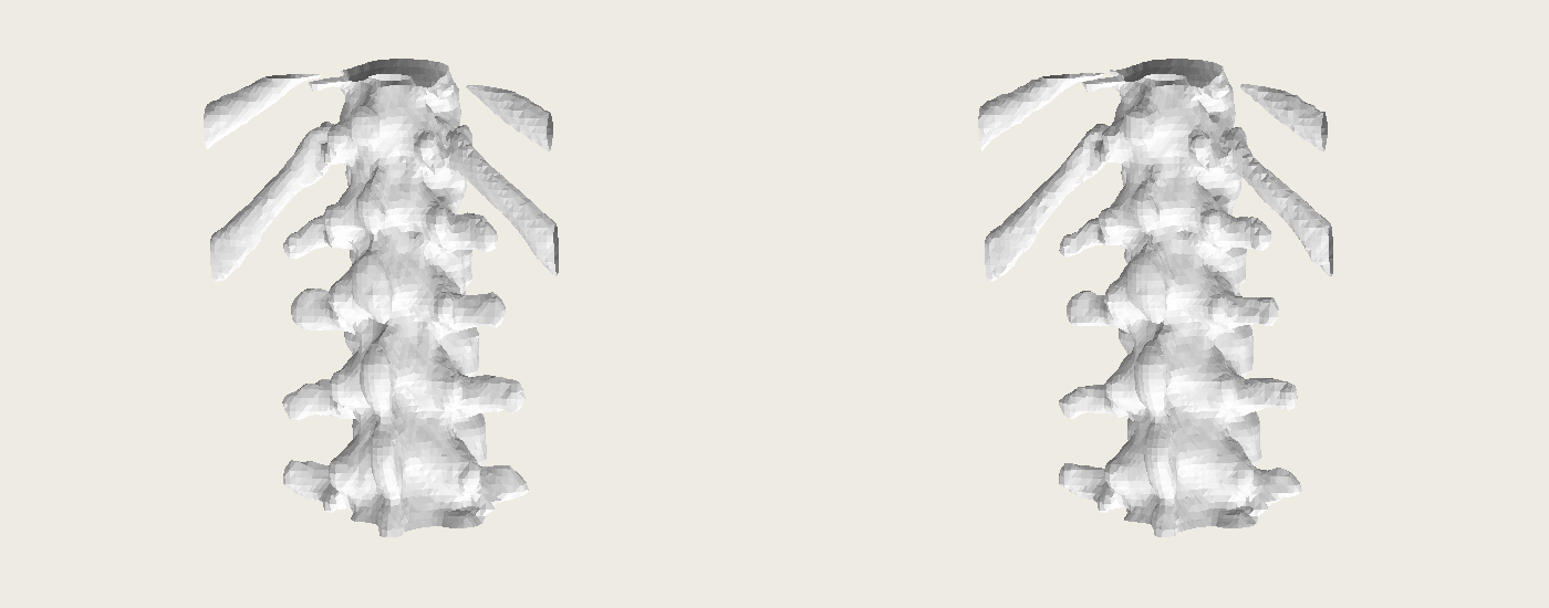
Drag either pane to rotate both. Shared radiograph lights: red view 1, green 17, blue 33. Detector planes retain fixed acquisition poses (20–55 keV, log window 0–8).
126 fitting views · 18 withheld views
Drag to rotate · Arrow keys to turn · + / − to zoom · Home to reset.Both volumes share a camera and material range. Radiograph colours affect surfaces only.
Distance from the first voxel centre along the selected grid axis, in millimetres. Rust: reconstructed · Blue: assigned reference
Acquisition, measurements and limitations
200,000 photons per ray integrated across three ideal channels.
- Inverse grid
- 64 × 64 × 64 voxels (Z, Y, X)
- Voxel spacing
- 2.326 × 2.326 × 3.000 mm (X, Y, Z)
- Bone fraction RMSE
- 0.03326
- Water fraction RMSE
- 0.03917
- Convergence established
- No
- Assigned material phantom. Fractions are not measured patient composition.
- 1,000-update budget reached. Stationarity and noise-limited performance are not established.
- Vertebral region includes cropped ribs. Source-header laterality is not independently established.
- Reference and recovered arrays share the inverse grid. Surfaces remain unsmoothed and open at cropped boundaries.
Rister et al. CT-ORG (2019), case 2 bone labels, cropped, assigned and volume averaged · SpekPy 2.5.4 spectrum generator · Hubbell and Seltzer, NIST SRD126, the water coefficient source used for simulation · NIST SRD126 ICRU-44 cortical bone coefficient source used for simulation
Coordinates are in the recorded object frame. Anatomical laterality is not asserted. Clipped surfaces stay open. The interactive camera uses perspective and the static plate uses orthographic projection. Surface lighting and volume opacity serve inspection. The slice and profile values come from the recorded fields.
20–55 keVWithheld view 5
Simulated observation

Black 0 · white 8
Generating expectation

Black 0 · white 8
Withheld-view prediction

Black 0 · white 8
Observation − prediction (Poisson scaled)

Blue -5 · pale 0 · red 5
Display clipping in this channel
- Simulated observation: 1555 below the window, 1 above, 0 masked.
- Generating expectation: 3119 below the window, 0 above, 0 masked.
- Withheld-view prediction: 3119 below the window, 0 above, 0 masked.
- Observation − prediction (Poisson scaled): 27 below the window, 75 above, 0 masked.
Clipping affects the image display only.
55–80 keVWithheld view 5
Simulated observation

Black 0 · white 5.5
Generating expectation

Black 0 · white 5.5
Withheld-view prediction

Black 0 · white 5.5
Observation − prediction (Poisson scaled)

Blue -5 · pale 0 · red 5
Display clipping in this channel
- Simulated observation: 1550 below the window, 0 above, 0 masked.
- Generating expectation: 3119 below the window, 0 above, 0 masked.
- Withheld-view prediction: 3119 below the window, 0 above, 0 masked.
- Observation − prediction (Poisson scaled): 43 below the window, 26 above, 0 masked.
Clipping affects the image display only.
80–120 keVWithheld view 5
Simulated observation

Black 0 · white 4
Generating expectation

Black 0 · white 4
Withheld-view prediction

Black 0 · white 4
Observation − prediction (Poisson scaled)

Blue -5 · pale 0 · red 5
Display clipping in this channel
- Simulated observation: 1588 below the window, 16 above, 0 masked.
- Generating expectation: 3119 below the window, 8 above, 0 masked.
- Withheld-view prediction: 3119 below the window, 0 above, 0 masked.
- Observation − prediction (Poisson scaled): 3 below the window, 0 above, 0 masked.
Clipping affects the image display only.
Residual: (observation − prediction) / √max(predicted count, 1). Positive values mean more observed photons than predicted. The entire view was withheld from fitting.
Recorded data and display
96 × 96 detector samples, displayed at their physical aspect ratio. The extent is384 × 384 mm. Full detector cell-face extent in centred detector coordinates. These are the original selected samples. Enlargement adds no detector resolution.
Assigned CT-derived material phantom with simulated independent Poisson channels: finite-budget reconstruction, not measured patient composition.
Observation display: -log((counts+0.5)/open_beam);0.5 is a display-only continuity correction. Residual display: (observed-predicted)/sqrt(max(predicted,1)); limits[-5,5].
Original data and attribution · Display records · Source identities
Throughout this chapter, someone else chose the acquisition. Chapter 13 makes that choice part of the problem: which next view, and which allocation of exposure, would improve a specified registration or reconstruction task?
References
- Siddon, Robert L. (1985). Fast calculation of the exact radiological path for a three-dimensional CT array. Medical Physics, 12(2), 252-255. https://doi.org/10.1118/1.595715
- Momeni, Mohammadhossein, Gopalakrishnan, Vivek, Dey, Neel, Golland, Polina and Frisken, Sarah (2024). Differentiable Voxel-based X-ray Rendering Improves Sparse-View 3D CBCT Reconstruction. arXiv. https://doi.org/10.48550/arXiv.2411.19224
- Alvarez, R. E. and Macovski, A. (1976). Energy-selective reconstructions in X-ray computerised tomography. Physics in Medicine and Biology, 21(5), 733-744. https://doi.org/10.1088/0031-9155/21/5/002
- Alvarez, Robert (2017). Conditions for the invertibility of dual energy data. arXiv. https://doi.org/10.48550/arXiv.1711.10836
- Barzilai, Jonathan and Borwein, Jonathan M. (1988). Two-Point Step Size Gradient Methods. IMA Journal of Numerical Analysis, 8(1), 141–148. https://doi.org/10.1093/imanum/8.1.141