When the X-ray changes but the object has not moved
Exposure, spectrum and detector response can change an image without any object motion. An optimiser that cannot account for them may move the object to explain the wrong cause.
The object has not moved, yet the next image is brighter. Perhaps more photons were emitted. Perhaps the detector gain changed. Perhaps the display software has helpfully decided that yesterday’s greyscale was insufficiently dramatic. A pose optimiser supplied with a fixed intensity model can respond to all three by moving the anatomy.
The difficulty extends beyond brightness. A different spectrum changes the relative transmission through thick and thin regions. Scatter fills in contrast. Blur spreads an edge across neighbouring pixels. Some of these changes resemble motion closely enough that reducing image error can increase pose error.
A useful acquisition model keeps photons, detector signal and processed greyscale in their own units. It also needs observations that distinguish an acquisition change from a pose change. Otherwise the fit can trade one against the other while leaving the predicted image unchanged.
The code now needs to expose those acquisition assumptions. We will extend the pose evaluator from Chapter 6 with named calibration parameters and multiple views, while retaining its fixed pose chart and optimiser. SpectralPoseEvaluator supplies this composition. Its material and spectral calculations are developed in Chapter 8. Here the question is which quantities a fit is allowed to change, and what evidence could distinguish them.
7.1 Separate motion from acquisition changes
Let describe the rigid object pose and let collect acquisition parameters. These may include exposure, spectrum, scatter, detector response and processing settings. They are called nuisance parameters because pose is the quantity we want, not because the underlying physics is optional.
For a detector with a fixed count-to-signal gain, a linear mean model is
In equation (7.1), and are expected primary and scatter counts at unit exposure, is a relative exposure, is a linear spatial response, is gain in signal units per count, and is a uniform offset in signal units. The parameters describe the remaining acquisition conditions. Spatially varying gains and offsets can replace the scalars when calibration supports them.
The equation describes a mean. It does not specify the distribution of an observation or the order in which random detector events occur. Those details determine noise covariance. Subsequent nonlinear processing acts on the random observation, and its expected output need not equal the same processing applied to .
Keeping the stages separate prevents several unit errors. Scatter counts can be added to primary counts before conversion to signal. An electronic offset is added in signal units. An offset measured after logarithmic processing belongs to another domain again. A single additive term cannot move between these locations without changing its meaning.
Near a reference pose and acquisition, the first-order change in the predicted image is
The two contributions in equation (7.2) can point in similar image directions. An intensity change is not necessarily harmless to pose recovery merely because its physical cause is non-geometric. What matters is whether the pose Jacobian can reproduce it on the observed region.
For now we keep the object attenuation field fixed. Deformation or a change in material composition requires a scene parameter as well. Assigning those effects to acquisition would conceal a different modelling error.
7.2 Exposure, gain and offsets
Fluence and gain can produce the same mean brightness change while producing different noise changes. Let and let the recorded signal be , where the independent electronic noise has zero mean and variance . Then
Doubling exposure in equation (7.3) doubles both the photon-dependent mean above offset and the photon variance in signal units. Doubling gain doubles that mean but multiplies the photon variance by four (Figure 7.1). From the mean alone, only the product is identifiable. Repeated calibrated measurements and an adequate noise model can supply additional information.
Reference
20 photons on average · 1 signal unit per photon
- Mean
- 20.004 (20 exact)
- Variance
- 20.104 (20 exact)
Double exposure
40 photons on average · 1 signal unit per photon
- Mean
- 40.016 (40 exact)
- Variance
- 40.253 (40 exact)
Double gain
20 photons on average · 2 signal units per photon
- Mean
- 39.98 (40 exact)
- Variance
- 80.384 (80 exact)
131,072 independent draws per condition, with zero offset and read noise. The doubled gain allows only even signal values.
Figure data
Numerical examples recorded on 9 September 2026. Sources and calculation records.
Dark observations constrain electronic offsets and readout noise. Open-beam observations constrain the spatial response to illumination, but their interpretation still depends on exposure and spectrum. A flat field taken under a different spectrum may not calibrate material-dependent transmission under the new spectrum.
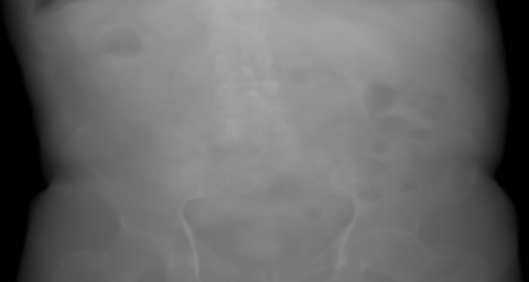
Region in the synthetic AP projection
Expected patch

10 counts

Relative Poisson SD: 31.6%
100 counts

Relative Poisson SD: 10.0%
1,000 counts

Relative Poisson SD: 3.2%
10,000 counts

Relative Poisson SD: 1.0%
The same 32 × 32 pixel patch at four exposure levels. Counts are actual recorded draws from the canonical Poisson sampler. Each level has a distinct observation identifier. The expected background is defined by the patch's four-pixel border.
Image model and data
These are simulated primary radiographs of three generated MAISI CT candidates, not patient acquisitions. The full native CT supplies attenuation through the stated water-equivalent approximation at 80 keV. No scatter, spectrum or material-specific calibration is included. AP and PA are cone-beam views and need not be exact horizontal mirrors.
Radiographs use a common optical-depth display interval 0–8. The 480 × 256 detector spans 600 × 480 mm: its pixels have unequal pitches, so the displayed physical aspect is 5:4. No clinical left/right mirror is applied. A/P/R/L/S/I mark body-relative directions.
The patch spans 40 × 60 mm and is displayed at that physical aspect. Every noise image uses the same inverse normalised-count window 0.8–1.2. Values outside it saturate only in the display. Relative Poisson standard deviations are exact model values, not estimates from these four images.
All 39 distinct projections were checked at 4,096 and 8,192 samples per ray, with three independent reference rays per view. The larger rotation study retains one-degree steps without interpolating between images. Playback timing is illustrative.
Geometry, observations and numerical checks · Source and output digests
CalibrationSpec turns the mean-model ambiguity into an interface constraint. The input to calibrate is an expected detector response, after any declared spatial spread, and its output is gain times exposure times that response, plus the electronic offset. The output unit is required because a count image and an image in detector signal units admit different observation models. The low-level operator allows a fixed calibration map to vary across pixels, but an optimised gain or offset must be a shared scalar.
@dataclass(frozen=True, slots=True)
class CalibrationSpec:
    """y = gain * exposure * mean + offset, in the declared output unit.

    Gain is strictly positive; exposure is non-negative; offset is any finite
    electronic baseline. A fixed flat-field may vary by pixel. Optimised gain
    and offset are shared scalars: unconstrained correction images are excluded.
    Exposure and gain cannot both be active because their scale is unidentifiable.
    """

    output_unit: str
    shared_gain: bool = True
    shared_offset: bool = True
    active_mean: bool = True
    active_gain: bool = False
    active_exposure: bool = False
    active_offset: bool = False

    def __post_init__(self) -> None:
        if not self.output_unit.strip():
            raise ContractError("calibration output unit is required")
        for name in (
            "shared_gain",
            "shared_offset",
            "active_mean",
            "active_gain",
            "active_exposure",
            "active_offset",
        ):
            if type(getattr(self, name)) is not bool:
                raise ContractError(f"{name} must be a boolean")
        if self.active_gain and self.active_exposure:
            raise ContractError("fix gain or exposure before fitting the other scale")
        if self.active_gain and not self.shared_gain:
            raise ContractError("a fitted gain must be a shared acquisition parameter")
        if self.active_offset and not self.shared_offset:
            raise ContractError("a fitted offset must be a shared acquisition parameter")
The rejection of simultaneously active exposure and gain follows directly from equation (7.3): their image derivatives cannot separate the two factors from the mean. The code therefore makes the caller fix one. Allowing both and waiting for the optimiser to discover the null direction would merely make the same identifiability calculation more expensive. A fitted per-pixel correction is excluded for a related reason: it could consume the residual that is supposed to constrain pose.
Exposure controls may alter more than photon number. AAPM Task Group 125 describes fluoroscopic control systems that adjust tube potential, current, pulse width and filtration. Similar displayed brightness can therefore accompany different spectral and temporal conditions. The recorded acquisition settings help distinguish these changes from a scalar gain adjustment. [17]
When scale and offset are uncertain but spatial response is otherwise modelled, fit an affine correction to the predicted image. Let be a fixed-domain image prediction, and use fixed positive weights :
The scale in equation (7.4) is an image-domain nuisance coefficient, and it need not separately identify exposure or detector gain. With weights independent of , and pose, this is a weighted least-squares problem. Weights computed once from observed counts remain fixed in this solve. Weights updated from the predicted counts or other fitted parameters instead require differentiating that dependence or declaring a frozen-weight approximation.
Write weighted means as and . Differentiating with respect to the offset gives . Substitution leaves a one-parameter regression whose unconstrained minimiser is
The denominator in equation (7.5) must be positive. A constant predicted image cannot separately identify scale and offset. If the unconstrained scale is nonpositive, it is outside the stated model, so use a specified positive lower bound and solve the corresponding constrained problem.
This elimination of nuisance parameters is called profiling. At each pose, use the best admissible scale and offset, then compare poses through the resulting objective. For an interior solution and a nonconstant observation, the profiled discrepancy can be written using weighted correlation :
Equation (7.6) shows exactly which discrepancies the fit removes. Among poses with positive correlation, minimising this objective gives the same ordering as maximising weighted correlation. The factor multiplying depends only on the fixed observations and weights. A negative correlation would also look favourable after squaring, which is why the positive-scale condition cannot be discarded.
A spatially uniform offset may represent a calibrated electronic bias. It cannot generally represent scatter, heel-effect variations or a spatially varying detector response. Their images need not be affine copies of the prediction.
Profiling is available mathematically under the assumptions just derived. The library’s recovery adapter instead fits the declared scale and offset jointly with pose. This permits named groups to share a parameter across views and permits explicit calibration priors. It does not evaluate equation (7.5) at each trial, so a result from that adapter must be described as a joint fit rather than an affine-profiled one.
7.3 Spectrum, filtration and beam hardening
A scalar exposure changes how many incident photons are available. A spectral change also changes how strongly different material paths attenuate them.
For a single homogeneous material of path length in millimetres, collect the incident spectrum and the relevant nonnegative linear detector weighting into normalised weights . With , and fixed attenuation coefficients in , the normalised expected transmission is
The averaging in equation (7.7) occurs before the logarithm. The weights can describe photon counts or a linear energy-weighted mean, provided numerator and open-beam normalisation use the same response. They do not turn an energy-integrating detector into a Poisson counter.
Define the transmitted weights . They sum to one and shift towards components with smaller attenuation as the material thickens. Differentiating the effective optical depth gives
In equation (7.8), the slope is the attenuation averaged over the transmitted components. Its derivative is minus their variance. The log signal is therefore concave in homogeneous path length, with a constant slope only when all nonzero-weight components have the same attenuation. In ordinary diagnostic spectra this preferential removal of more strongly attenuated components commonly shifts the transmitted spectrum towards higher energies: beam hardening.
For an exact two-component example, take equal incident weights and attenuation coefficients and . The arithmetic of the mixture gives the values in Table 7.1, including the discrepancy from using the incident mean coefficient.
| Path length (mm) | Transmission | Effective optical depth | Optical depth from the incident mean coefficient |
|---|---|---|---|
| 0 | 1 | 0 | 0 |
| 50 | 0.414830 | 0.879885 | 1 |
| 100 | 0.208833 | 1.566219 | 2 |
Doubling the path from 50 to 100 mm does not double the effective optical depth (Figure 7.3). An effective coefficient fitted to the thinner path consequently overpredicts attenuation through the thicker one. A pose fit can partly hide that error by shortening thick paths, thereby making a spectral error look like a geometric correction.
Effective optical depth bends below the incident-mean line
- −log T
- Incident mean: 0.02 ℓ
The weakly attenuated component takes over
- μ₁ = 0.01 mm⁻¹
- μ₂ = 0.03 mm⁻¹
The slope falls from 0.02 to 0.01036 mm⁻¹ over this interval. Log signals and fractions are derived from the recorded component means.
Figure data
Numerical examples recorded on 9 September 2026. Sources and calculation records.
With several materials, the energy-dependent optical depth is a sum of their material path lengths weighted by their attenuation coefficients:
The material dependence in equation (7.9) prevents a single global scale from correcting every ray after a spectral change. Two rays with equal transmission under one spectrum can respond differently to another if their material compositions differ. Filtration changes the incident weights, and object attenuation then changes the transmitted weights separately on every path.
Estimating an arbitrary spectrum from one projection of uncertain anatomy is usually underdetermined. A low-dimensional spectral model, recorded acquisition settings and independent material-thickness information constrain a more interpretable problem. Chapter 8 develops the spectral and detector integration needed to evaluate such a model.
7.4 Scatter and background structure
Scatter adds photons that have changed direction within the object or surrounding scene. Its spatial distribution depends on illumination, material, geometry and detector acceptance. It is not generally a constant veil, although a slowly varying approximation can be useful over a restricted region. [2]
For local primary signal and approximately unchanged scatter signal across a small feature, a primary difference has observed relative contrast
The factor in equation (7.10) quantifies the dilution. If , the contrast is halved. This argument assumes the scatter contribution is effectively equal on the two sides of the feature, and it does not assert that scatter is uniform across the whole detector.
In a count-domain model with open-beam mean , primary optical depth and additive mean scatter , write
The derivative in equation (7.11) holds and fixed. It shows why scatter changes more than the baseline of a log projection: it reduces sensitivity to changes in the primary optical depth. When pose also changes scatter, the full pose derivative includes that additional dependence.
A smooth background model can use a small set of detector basis functions. With denoting their values, write
Equation (7.12) can describe broad variation with relatively few coefficients. Nonnegative basis functions with nonnegative coefficients are one way to enforce the sign condition. This is an image approximation. The coefficients do not separately identify the scattering events that produced the signal.
Giving every pixel an unconstrained additive correction would let the correction reproduce every residual. Even nonnegative per-pixel scatter can explain a large class of positive discrepancies and weaken pose recovery. Restricting spatial bandwidth, bounding magnitude from calibration or tying the background across acquisitions reduces this freedom.
A change in collimation supplies useful physical evidence because it changes the illuminated material that produces scatter. Cropping an already acquired image removes pixels from analysis but leaves the photons that reached the retained pixels unchanged. Cropping therefore cannot reproduce the scatter reduction from physical collimation.
The present spectral recovery composition contains primary signal, optional fixed spatial response and electronic calibration. It has no fitted scatter field. An externally supplied additive image would remain a prescribed background until a transport calculation or calibration justified calling it scatter. Chapter 9 supplies complete-history detector scores, which include both primary and scattered arrivals, so adding that total to an existing primary image would count the primary twice.
7.5 Detector blur, noise and processing
A blur operator acts differently depending on where it enters image formation. A deterministic filter applied after photon detection mixes already random pixel values. A detector that spreads each photon’s charge over several pixels generates a correlated response event by event. Both can have a similar mean blur while requiring different noise models.
For a definite post-detection model, let independent Poisson counts have mean vector , and let the output be , with independent zero-mean electronic noise of covariance . Then
The off-diagonal entries in equation (7.13) arise when output pixels share input counts. Treating those outputs as independent Poisson counts would change both their variance and their dependence. This formula assumes is deterministic and that electronic noise is added after the filter. A different order changes its covariance contribution.
Blur can also couple directly to pose. Consider a one-dimensional sharp feature and a blur kernel whose centroid is displaced by , so that . Convolution gives
Only the sum appears in equation (7.14). A free kernel shift and a geometric image shift are exactly confounded in this model. Fixing the kernel centroid from calibration removes that freedom. Estimating blur width can still be useful, but width and centroid have different geometric consequences.
The identical profiles in Figure 7.4 make this ambiguity explicit.
Move the feature by one pixel
- Original feature
- Feature displaced +1 px
The two filtered profiles coincide
- Feature +1 px, fixed kernel
- Fixed feature, kernel +1 px
Fixed stencil: [0, 0.125, 0.75, 0.125, 0]. Its array shifts by −1 to displace the output by +1 pixel under the recorded indexing convention. The feature stays clear of the image edges.
Figure data
Numerical examples recorded on 9 September 2026. Sources and calculation records.
For nonlinear processing , a first-order covariance approximation around the mean is
Equation (7.15) requires a differentiable processing map and fluctuations small enough for its local linearisation. Clipping violates that approximation at the clipping boundary and removes local intensity sensitivity in saturated regions. A log transform is also poorly approximated by a first-order expansion near zero.
Temporal filtering introduces another coupling. A displayed fluoroscopic frame may combine observations from several earlier poses. Rendering one instantaneous pose and fitting it to that mixture can place an edge between positions the anatomy actually occupied. If timing and temporal response are known, predict the exposure-weighted sequence or blur over motion. Otherwise the frame does not supply an unambiguous instantaneous-pose observation.
For digital X-ray objects, DICOM distinguishes FOR PROCESSING from FOR PRESENTATION images. FOR PROCESSING images already include detector corrections, while an ORIGINAL image intended for presentation may include operations such as unsharp masking. These labels do not specify the full processing sequence. Establish that sequence before choosing the measurement likelihood. [5]
7.6 Jointly estimate pose and nuisance parameters
Suppose a fixed whitening transform has placed both the residual and its Jacobians in noise-normalised coordinates. Write the current residual as , the pose Jacobian as and the nuisance Jacobian as . Local increments solve
The pose variable in equation (7.16) uses the dimensionless scaling from Chapter 6. Scale nuisance coordinates sensibly as well. A log-gain increment, for example, describes a relative multiplicative change while keeping gain positive.
CalibrationBlock gives those coordinates a fixed meaning for an entire solve. A view names its calibration group: views carrying the same name use the same gain, exposure and offset. An active positive scale is its reference value multiplied by exp(scale_step * z). An active offset is its reference plus offset_step * z, in the declared signal unit. The parameter vector begins with the six scaled pose coordinates and then contains these named nuisance blocks in their declared order.
@dataclass(frozen=True, slots=True)
class CalibrationBlock:
    """Named acquisition group sharing one gain/exposure/offset across its views.

    Exactly one multiplicative scale may be fitted. Its positive chart is
    reference*exp(scale_step*z); the other scale is fixed to remove the gain /
    exposure gauge. An active offset is reference+offset_step*z in output units.
    Optional Gaussian priors act on these dimensionless chart coordinates.

    Device parameters are rounded to binary32. The VJP differentiates the smooth
    physical chart at those represented values, not the discontinuous rounding
    map. Shared physical derivatives stay binary64 until the chart product is
    formed, so a large positive scale can preserve a small logarithmic partial.
    """

    name: str
    gain: float = 1.0
    exposure: float = 1.0
    offset: float = 0.0
    fit_scale: Literal["none", "gain", "exposure"] = "none"
    fit_offset: bool = False
    scale_step: float = 1.0
    offset_step: float = 1.0
    scale_prior_precision: float = 0.0
    offset_prior_precision: float = 0.0

    def __post_init__(self) -> None:
        if not self.name.strip():
            raise ContractError("calibration groups need non-empty names")
        if self.fit_scale not in ("none", "gain", "exposure") or type(self.fit_offset) is not bool:
            raise ContractError("invalid calibration activity specification")
        for name in ("gain", "exposure", "scale_step", "offset_step"):
            if finite_scalar(getattr(self, name), name, minimum=0) <= 0:
                raise ContractError(f"{name} must be strictly positive in the recovery chart")
        finite_scalar(self.offset, "offset")
        for name in ("scale_prior_precision", "offset_prior_precision"):
            finite_scalar(getattr(self, name), name, minimum=0)
        if self.fit_scale == "none" and self.scale_prior_precision:
            raise ContractError("a scale prior requires an active scale")
        if not self.fit_offset and self.offset_prior_precision:
            raise ContractError("an offset prior requires an active offset")
        for name in ("gain", "exposure", "offset"):
            try:
                _physical_parameter(getattr(self, name), name, positive=name != "offset")
            except NumericalError as error:
                raise ContractError(str(error)) from error

    @property
    def dimension(self) -> int:
        return int(self.fit_scale != "none") + int(self.fit_offset)

    def decode(self, coordinates: Vector) -> tuple[float, float, float]:
        if len(coordinates) != self.dimension:
            raise ContractError("nuisance coordinates differ from the declared group chart")
        if not all(math.isfinite(value) for value in coordinates):
            raise NumericalError("trial nuisance coordinates are non-finite")
        gain, exposure, offset = self.gain, self.exposure, self.offset
        cursor = 0
        if self.fit_scale != "none":
            try:
                scale = math.exp(self.scale_step * coordinates[cursor])
            except OverflowError as error:
                raise NumericalError("trial logarithmic calibration scale overflowed") from error
            if self.fit_scale == "gain":
                gain *= scale
            else:
                exposure *= scale
            cursor += 1
        if self.fit_offset:
            offset += self.offset_step * coordinates[cursor]
        return (
            _physical_parameter(gain, "gain", positive=True),
            _physical_parameter(exposure, "exposure", positive=True),
            _physical_parameter(offset, "offset"),
        )

    def gradient(self, coordinates: Vector, physical_gradient: Vector) -> Vector:
        if len(physical_gradient) != 3:
            raise ContractError("a calibration gradient needs gain, exposure and offset partials")
        gain, exposure, _ = self.decode(coordinates)
        gradient: list[float] = []
        if self.fit_scale != "none":
            index, value = (0, gain) if self.fit_scale == "gain" else (1, exposure)
            gradient.append(_scaled_product(self.scale_step, value, physical_gradient[index]))
        if self.fit_offset:
            gradient.append(_scaled_product(self.offset_step, physical_gradient[2]))
        return tuple(gradient)

    def prior(self, coordinates: Vector) -> Evaluation:
        if len(coordinates) != self.dimension:
            raise ContractError("prior coordinates differ from calibration chart")
        precisions = () if self.fit_scale == "none" else (self.scale_prior_precision,)
        precisions += (self.offset_prior_precision,) if self.fit_offset else ()
        return Evaluation(
            math.fsum(0.5 * p * z * z for p, z in zip(precisions, coordinates, strict=True)),
            tuple(p * z for p, z in zip(precisions, coordinates, strict=True)),
        )
The gradient method supplies the chart’s chain factors. A derivative with respect to physical gain must be multiplied by the represented gain and scale_step before it becomes a derivative with respect to z. This multiplication retains binary64 range: storing a very small physical partial in binary32 first could erase it before a large gain made its chart derivative useful. Device calibration values themselves use binary32. As with the earlier operators, the derivative describes the smooth physical calculation at those represented values, not the discontinuous map that rounds a real number into storage.
Optional prior precisions penalise the dimensionless coordinates relative to their references. They are added once per group, however many views share that group. Such a prior supplies additional information, and its effect must remain distinguishable from information supplied by the images.
For full-column-rank and unconstrained local nuisance increments, minimisation over the nuisance coordinates gives
Substituting equation (7.17) into the local objective removes the image directions that nuisance changes can fit. The remaining pose curvature is
The matrix in equation (7.18) is the Schur complement of the nuisance block in the joint normal equations. It gives the local data information left for pose after nuisance fitting. If a pose-induced image direction lies entirely in the column space of , the nuisance fit can absorb it and the corresponding information vanishes. Rank-deficient nuisance models require a pseudoinverse or an identifiable reparameterisation, and active constraints require the corresponding constrained local problem.
For one pose direction with image derivative and one nuisance direction , define their cosine , with both vectors nonzero. The remaining information reduces to
In equation (7.19), orthogonal effects leave pose information unchanged. At , only 19% of the information remains, and at , only 1.99% remains. A nuisance parameter can be physically reasonable and still make pose substantially harder to estimate.
Figure 7.5 shows how quickly the remaining information falls as the two effects become parallel.
Information remaining after fitting one nuisance direction
- c = 0
- 100% remains
- c = 0.9
- 19% remains
- c = 0.99
- 1.99% remains
Figure data
Numerical examples recorded on 9 September 2026. Sources and calculation records.
Calibration supplies information about nuisance quantities independently of the registration image. In a quadratic local model with nuisance precision , the effective pose curvature becomes
provided the matrix being inverted is positive definite. Equation (7.20) interpolates between freely fitted nuisance quantities and strongly constrained calibration. Its extra curvature comes from the calibration or prior. It should not be attributed entirely to the registration image.
Multiple acquisitions can share an object pose while having separate exposures, or share detector response parameters while containing different known object poses. Sharing a parameter forces one value to explain every view in its group. Different viewing geometries can make a pose change and that nuisance change produce distinguishable collections of image changes, even when their effects overlap in one view. In the local analysis above, combine the views by stacking their residuals and Jacobian rows while keeping one column for each shared parameter. Write those dependencies before fitting. If every image has both a free exposure and a free scalar detector gain, their products remain confounded in the means. Adding images with the same freedom does not resolve it.
The implemented multi-view problem takes the first of those arrangements: every SpectralView observes one shared object-to-world pose through its own fixed source and detector geometry. Each view also declares its observation domain and calibration group. Material fractions, coefficient tables, energy weights, detector response and any blur stencil remain fixed. This is enough to ask whether a pose estimate changes when a constrained calibration error is allowed to explain brightness, but it cannot infer an unknown spectrum or a moving object independently in each view.
    def __call__(self, parameters: Vector) -> Evaluation:
        require_no_tape()
        if self._running:
            raise ContractError("a spectral evaluator cannot be used concurrently or recursively")
        if len(parameters) != self.dimension:
            raise ContractError("parameter count differs from pose and calibration charts")
        pose = self.chart.pose(parameters[:6])
        decoded = tuple(
            block.decode(parameters[section])
            for block, section in zip(self.problem.calibration, self._group_slices, strict=True)
        )
        ctx, wp = self.context, self.context.wp
        self._running = True
        self.last_view_losses = None
        try:
            with ctx.scope():
                try:
                    self._clear_statuses()
                    self._pose_values[:] = pose.packed()
                    self._parameter_values[:] = tuple(value for block in decoded for value in block)
                    wp.copy(self._pose_device, self._pose_host, stream=ctx.stream)
                    wp.copy(self._parameters_device, self._parameters_host, stream=ctx.stream)
                    for item in self._prepared:
                        view = item.view
                        gain, exposure, offset = self._parameter_views[item.group]
                        project_material_paths(
                            self._pose_device,
                            workspace=item.material,
                            stream=ctx.stream,
                            validate=False,
                        )
                        spectral_signal(
                            item.material.paths,
                            view.coefficients,
                            view.weights,
                            view.response,
                            out_mean=item.mean,
                            workspace=item.spectral,
                            stream=ctx.stream,
                            validate=False,
                        )
                        if item.blur is not None:
                            blur(
                                item.mean,
                                out_signal=item.spread,
                                workspace=item.blur,
                                stream=ctx.stream,
                                validate=False,
                            )
                        calibrate(
                            item.spread,
                            gain,
                            exposure,
                            offset,
                            out_signal=item.prediction,
                            spec=item.calibration_spec,
                            workspace=item.detector,
                            stream=ctx.stream,
                            validate=False,
                        )
                        evaluate_objective(
                            item.prediction,
                            view.observation,
                            out_loss=item.loss,
                            out_seed=item.image_seed,
                            weights=view.objective_weights,
                            workspace=item.objective,
                            stream=ctx.stream,
                            validate=False,
                        )
                        calibration_vjp(
                            item.spread,
                            gain,
                            exposure,
                            offset,
                            seed=item.image_seed,
                            out_grad_mean=item.spread_seed,
                            out_grad_gain=item.nuisance_gradients[0]
                            if item.calibration_spec.active_gain
                            else None,
                            out_grad_exposure=item.nuisance_gradients[1]
                            if item.calibration_spec.active_exposure
                            else None,
                            out_grad_offset=item.nuisance_gradients[2]
                            if item.calibration_spec.active_offset
                            else None,
                            spec=item.calibration_spec,
                            workspace=item.detector,
                            stream=ctx.stream,
                            validate=False,
                        )
                        if item.blur is not None:
                            blur_transpose(
                                item.spread_seed,
                                out_grad_signal=item.mean_seed,
                                workspace=item.blur,
                                stream=ctx.stream,
                                validate=False,
                            )
                        spectral_vjp(
                            item.material.paths,
                            view.coefficients,
                            view.weights,
                            view.response,
                            seed=item.mean_seed,
                            out_grad_paths=item.material.adj_paths,
                            workspace=item.spectral,
                            stream=ctx.stream,
                            validate=False,
                        )
                        material_projection_vjp(
                            self._pose_device,
                            workspace=item.material,
                            out_pose=item.pose_gradient,
                            stream=ctx.stream,
                            validate=False,
                        )
                    wp.copy(self._control_host, self._control_device, stream=ctx.stream)
                    wp.copy(self._nuisance_host, self._nuisance_device, stream=ctx.stream)
                finally:
                    # Rejected evaluations must finish using pinned staging before
                    # the optimiser can write the next trial into the same buffers.
                    wp.synchronize_stream(ctx.stream)
            self._check_statuses()
            return self._assemble(parameters)
        finally:
self._running = FalseRead the forward calls in order: material paths produce a spectral mean, the optional spatial operator spreads it, calibration converts it to the observation’s units, and the objective returns its image seed. The reverse calls follow those dependencies backwards. calibration_vjp separates nuisance derivatives from the image seed. blur_transpose returns that seed through the finite spatial response, and the spectral and material-projector VJPs finally return a pose derivative. _assemble weights and sums the view losses and pose derivatives in the fixed chart, and sums each nuisance derivative into its named group. No detector-by-parameter Jacobian is needed.
Preparation allocates the image buffers and validates immutable inputs. A trial transfers only pose and calibration values to CUDA, while losses, small gradients and status words return at a declared checkpoint. That is why the repeated calls use validate=False: each operator retains its shape and ownership checks while avoiding repeated scans of fixed inputs. It remains necessary to inspect numerical status before accepting the trial. The inner finally also matters. Pinned host memory can still be in use by an asynchronous copy when an exception occurs, so draining the owning stream prevents the next trial from overwriting it prematurely.
A count-domain Poisson objective has stricter entry conditions here: unit gain, zero offset, no fitted gain or offset, no spatial blur and a detection-probability response. A general calibrated signal uses a declared signal-domain discrepancy. The adapter cannot infer the correct likelihood from the fact that an array happens to be non-negative.
7.7 Controlled mismatch experiments
A useful mismatch experiment changes one physical cause while holding pose fixed. For exposure, keep geometry, spectrum and detector response fixed while changing incident fluence. For gain, keep the photon process fixed and change the signal conversion. These interventions have different variance predictions even when their mean images agree.
Begin with cases whose forward dependencies are explicit. The affine model isolates scale and offset. The two-component spectral model isolates path-dependent hardening. The shifted-kernel example isolates an exact blur-pose ambiguity. Each answers a specific question before several effects are combined.
For a nuisance condition and repeated observations indexed by , let be the recovered pose and the fixed reference. Express local left pose errors in a common coordinate system:
The errors in equation (7.21) use the same translation-first convention as the optimiser, with translational Lie coordinates in millimetres and rotation coordinates in radians. They describe bias locally when the errors lie within a consistent branch of the logarithm. Widely separated solutions should be reported as separate outcomes rather than averaged through a branch discontinuity.
Across repetitions, estimate the covariance of those local errors:
The mean error in equation (7.21) separates systematic displacement from the spread measured by equation (7.22). A model extension can reduce bias while increasing variance because it adds nuisance freedom. Reporting only a mean image loss hides that tradeoff. The experiments in Table 7.2 isolate acquisition changes while holding the physical pose fixed.
| Changed quantity at fixed pose | Quantities held fixed | Diagnostic comparison |
|---|---|---|
| Incident exposure | Spectrum, geometry, detector gain and processing | Mean and variance scaling and pose bias with and without exposure fitting |
| Electronic gain or offset | Incident photon distribution and geometry | Signal-domain calibration and affine-profiled pose |
| Spectral weights | Geometry, material paths and chosen open-beam normalisation | Residual dependence on material thickness and composition |
| Scatter-producing illumination | Object pose and detector settings | Broad residual structure and sensitivity to collimation |
| Spatial response | Geometry, photon process and kernel centroid where calibrated | Edge width, neighbouring-pixel covariance and pose variance |
| Temporal response | Known motion and acquisition timing | Difference between instantaneous and temporally integrated predictions |
A controlled comparison uses the same pose initialisation rule, fit region and stopping criteria across model variants. Otherwise a change in recovery can come from the optimiser’s opportunity to search rather than the added physics. Keep acquisition conditions used to select nuisance bounds separate from those used to assess the resulting model.
Repeated noise draws can be paired across model variants to compare their response to the same observation. The repetitions must still be independent across trials when estimating uncertainty from them. For acquired data, record the calibration, exposure timing and reference-pose uncertainty alongside the image: those observations determine what the experiment can distinguish.
The canonical driver, experiments/acquisition-mismatch/run.py, uses the evaluator in Listing 7.3 to compare fixed calibration with the declared joint fit, starting both from the same pose and calibration references. Fitting views supply the objective and derivatives. Held-out views are evaluated only after fitting, using the fitted groups without another calibration fit. Their losses therefore answer a predictive question rather than providing another opportunity to tune the model.
The driver records accepted parameters and termination reasons as well as fitting and held-out losses. Its inputs still determine what those records establish. In particular, a vacuum field has no pose-dependent attenuation: recovering a gain from its open-beam signal cannot demonstrate pose recovery. Spatially informative fields and independent geometric references are required for that claim. Source and input digests make an experiment traceable, but they cannot make an unidentifiable experiment informative.
7.8 Choose the next model term
Residual shape can suggest a missing mechanism, but it rarely identifies one uniquely. Broad positive residuals may indicate scatter, an offset or an underpredicted primary signal. Edge residuals may indicate pose, blur, deformation or a calibration error. Include a model term when a discriminating observation supports it and the fit constrains its effect.
The joint Jacobian provides a local test of that constraint. For a proposed nuisance derivative , remove the part already explained by the current model Jacobian :
where is the Moore–Penrose pseudoinverse. Equation (7.23) uses the same whitened image coordinates for both quantities. If , the new parameter has no distinct first-order image effect at this configuration. If it is small, calibration or another acquisition may be needed to separate its contribution.
This test is local. A nonlinear parameter can become distinguishable over a wider range of conditions, and an informative calibration exposure can reveal effects hidden in the anatomy image. Conversely, a numerically independent derivative is not enough to justify a physical interpretation if the proposed model does not describe the acquisition.
Compare extended models on observations that constrain the new term. Use calibrated dark and open-beam data for detector response, material-dependent observations for spectrum, and changes in illuminated volume for scatter. Evaluate residual structure, independent pose error and predictive performance under those conditions. A more flexible model will usually lower its fitting objective, but the question is whether its extra freedom predicts the changes the experiment actually imposed.
The next chapter follows the spectral calculation from the source, through material paths, to the detector-weighted signal. Scattering in Chapter 9 then adds photons whose routes through that scene are no longer the direct source-to-pixel segments.
References
- Rauch, Phillip, Lin, Pei-Jan Paul, Balter, Stephen, Fukuda, Atsushi, Goode, Allen, Hartwell, Gary, LaFrance, Terry, Nickoloff, Edward, Shepard, Jeff and Strauss, Keith (2012). Functionality and operation of fluoroscopic automatic brightness control/automatic dose rate control logic in modern cardiovascular and interventional angiography systems: A Report of Task Group 125 Radiography/Fluoroscopy Subcommittee, Imaging Physics Committee, Science Council. Medical Physics, 39(5), 2826-2828. https://doi.org/10.1118/1.4704524
- Dance, D. R., Christofides, S., Maidment, A. D. A., McLean, I. D. and Ng, K.-H. (eds.) (2014). Diagnostic Radiology Physics: A Handbook for Teachers and Students. Vienna: International Atomic Energy Agency. https://www.iaea.org/publications/8841/diagnostic-radiology-physics
- DICOM Standards Committee (2026). DICOM PS3.3 2026c: Information Object Definitions. National Electrical Manufacturers Association. https://dicom.nema.org/medical/dicom/current/output/chtml/part03/PS3.3.html