X-ray theory for non-radiologists
Radiographs, fluoroscopy and CT use the same underlying physics in different ways. This appendix explains the imaging quantities and conventions that the models in this book rely on.
Just as it’s not necessary to be Ansel Adams in order to be competent at rendering, you do not need to know everything a radiologist knows (or at least ought to know) in order to be proficient at differentiable photon transport. It does, however, help to speak the same language. The purpose of this appendix is to reach that same language, and the understanding that’s behind it.
An X-ray image is at the end of a measurement chain. An object attenuates the beam, a detector responds to the radiation that reaches it, and processing turns that response into a picture. Attenuation, transmitted radiation, detector output and displayed brightness have different units and statistics. A bright patch in a clinical image is not a material property you can copy into a renderer. To interpret it, you need to know how the image was acquired and processed.
This appendix covers projection radiography and fluoroscopy, then examines what a CT volume can tell us when we use it as input to a simulation. The aim is to give the data a physical meaning before we build a forward model or differentiate it.
A.1. What kind of X-ray image are we discussing?
In conventional diagnostic X-ray imaging, X-ray light travels from a source outside the patient, through the patient, to a detector. The detector records radiation, including photons that have scattered on the way and photons from all sorts of different and unrelated sources. Radiography does not observe anatomical surfaces directly but primarily observed the degree to which they absorb, scatter and modulate X-ray light. Radiography, fluoroscopy and CT use this arrangement in different ways, distinguished in Table A.1. [2, 3]
| Term | What is acquired or computed | What the resulting image represents |
|---|---|---|
| Radiograph | A projection exposure | A two-dimensional measurement in which structures along each source-to-detector path are superimposed |
| Fluoroscopy | A sequence of projection exposures, commonly using pulsed radiation | Time-resolved projection imaging, with acquisition and temporal processing that may change between frames |
| Computed tomography, or CT | Projection measurements from many directions | A reconstructed spatial estimate of attenuation-related properties |
| Cone-beam CT, or CBCT | Projections acquired using a cone-shaped beam and an area detector | A reconstructed volume, often acquired using a rotating gantry or C-arm |
| Digitally reconstructed radiograph, or DRR | A numerical projection of a volume | A simulated projection whose physical meaning depends on the forward model |
A DRR is computed from a model, the other images originate in detector measurements. That difference matters when deciding what a simulated pixel is supposed to represent.
In a projection, a foreground surface does not simply hide everything behind it as an opaque surface would in a visible-light image. In the primary-beam approximation, every traversed structure contributes to attenuation along the ray. A rib, a lung, a vertebral body and the operating table can all contribute to the same detector measurement.
At diagnostic energies, the refractive index of body materials is very close to unity. Conventional projection radiography uses no image-forming lens and usually neglects refraction: the useful contrast comes chiefly from transmission through the volume. X-ray lenses and mirrors do exist, but they are not how an ordinary radiograph forms its image. For its primary beam, the natural mathematical object is a line integral of attenuation, rather than a visible surface with a shading model. [2]
Light and dark deserve a moment of care. Photographic film is sensitive to X-rays, but conventional screen–film radiography usually records light produced by an intensifying screen. After development and fixing, exposed regions are darker and unexposed regions remain transparent. On an illuminated film negative, strongly attenuating structures appear lighter and are called radiopaque. This is radiopacity. Weakly attenuating structures are radiolucent. These are conventions for that presentation, not an immutable relationship between material and displayed grey level. [2] To prevent us from getting more confused than we need to, DICOM distinguishes the relationship between stored values and incident X-ray intensity from the transformations used to present those values. It keeps track of how we arrive at displayed pixels separately from how the stored signal relates to the radiation. [5]
Geometric phantom: one ellipsoid, two bone inserts and an air cavity.
Acquisition geometry
Static acquisition view. Interactive orbit controls load when available.
Attenuation image

Fixed display window: −log(mean T) from 0 to 4, where greater attenuation is brighter.
Magnification at the object centre 2.00×M = SDD / SOD
Drag to orbit the apparatus. Use the sliders to change acquisition geometry. Focal-spot averaging affects attenuation mode only.
Exact geometry and display assumptions
The surrounding ellipsoid has radii (55, 75, 40) mm and attenuation 0.02 mm⁻¹. Each bone insert uses 0.05 mm⁻¹ and the air cavity uses zero. These are stipulated coefficients at one energy, not calibrated material data. The inserts are disjoint and fully contained. Their coefficients replace the background over each inner chord.
Each detector pixel uses its centre ray. A nonzero focal spot uses 32 symmetric, equally weighted points on a disc: an approximation to a uniform finite source. Every sub-ray uses its exact finite-segment chord, and the image averages exp(−L), never L. Larger focal spots and magnifications can move features beyond the fixed detector. No random photons are sampled.
The detector has a fixed 320 mm square footprint with an 80 × 80 display sampling grid. The radiographic polarity and optical-depth window remain fixed as geometry changes. Surface shading is an illustrative directional-light rendering of the first intersected surface.
A.2. Anatomical directions and projection names
The second convention that we will need to wrap our heads around is directional terminology. Most of differentiability is about pose, and that of course presupposes a definition of what’s where.
Clinical directions are defined relative to the patient, not the monitor or the room. Anterior means towards the front of the body and posterior towards the back. Superior is towards the head and inferior towards the feet. Medial means towards the midline and lateral away from it. For a limb, proximal is nearer its attachment to the trunk and distal farther away. A patient lying face upwards is supine. A patient lying face downwards is prone.
The principal anatomical planes follow these directions. An axial or transverse plane divides superior from inferior portions. A coronal plane divides anterior from posterior portions, and a sagittal plane divides left from right. The midsagittal plane passes through the body’s midline. [4]
Projection names usually describe the beam’s direction through the patient. In an anteroposterior, or AP, projection, the beam enters anteriorly and exits posteriorly. A posteroanterior, or PA, projection reverses this direction. A lateral projection passes across the patient, while an oblique projection lies between the principal directions. These names express anatomical relationships, not a complete camera calibration.
In the standard DICOM coordinate system for a human patient, the positive axes point towards the patient’s left, posterior and head. This is commonly called LPS. Imaging and graphics libraries use other conventions, so a plausible-looking image may still be reflected or rotated incorrectly. DICOM records image position and orientation explicitly: array indices alone do not establish physical geometry. [5]
We will therefore endeavour to keep anatomical directions, patient coordinates, source coordinates, detector coordinates, and array indices distinct. “AP view” is useful clinical shorthand, but it cannot replace the transforms between those coordinate systems.
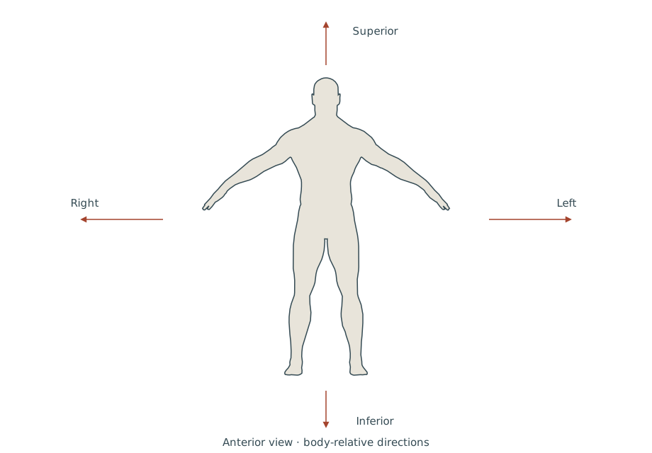
Static anterior view. Interactive controls load as the figure comes into view.
Chest request
AP
Anterior → posterior
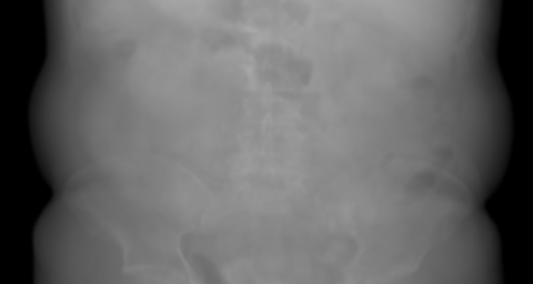
PA
Posterior → anterior
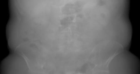
Right-to-left lateral
Right → left
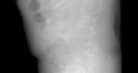
Lower thorax, abdomen and pelvis, rather than a full chest volume.
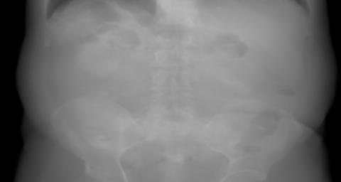
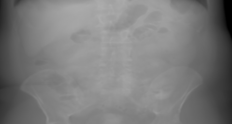
Abdomen request
AP
Anterior → posterior
PA
Posterior → anterior
Right-to-left lateral
Right → left
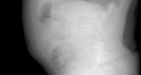
Abdomen and pelvis with lung bases.
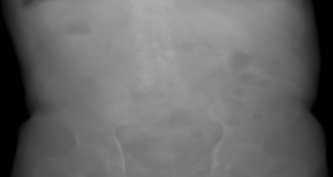
Pelvis request
AP
Anterior → posterior
PA
Posterior → anterior
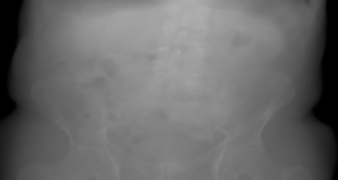
Right-to-left lateral
Right → left
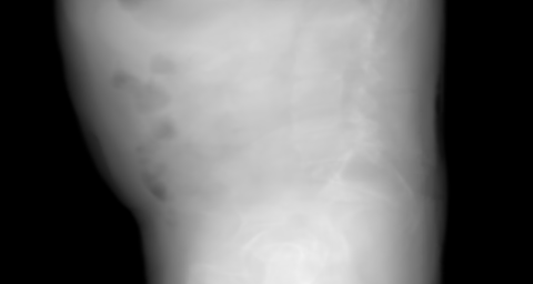
Abdomen and pelvis, including hips and lower spine, with the native inferior crop retained.
Image model and data
These are simulated primary radiographs of three generated MAISI CT candidates, not patient acquisitions. The full native CT supplies attenuation through the stated water-equivalent approximation at 80 keV. No scatter, spectrum or material-specific calibration is included. AP and PA are cone-beam views and need not be exact horizontal mirrors.
Radiographs use a common optical-depth display interval 0–8. The 480 × 256 detector spans 600 × 480 mm: its pixels have unequal pitches, so the displayed physical aspect is 5:4. No clinical left/right mirror is applied. A/P/R/L/S/I mark body-relative directions.
All 39 distinct projections were checked at 4,096 and 8,192 samples per ray, with three independent reference rays per view. The larger rotation study retains one-degree steps without interpolating between images. Playback timing is illustrative.
Geometry, observations and numerical checks · Source and output digests
The C-arm and its conventions
A C-arm carries the tube and detector at opposite ends of a C-shaped gantry. Ideally they move as a rigid pair. Orbital rotation moves the arm along its curved support, while angular rotation tilts the assembly about another mechanical axis. The relation of those axes to the patient depends on how the unit is positioned. In an isocentric system, the central ray passes through a common point, the isocentre, as the gantry rotates. Not every mobile C-arm maintains that geometry. [2]
Interventional projection names describe the detector’s position relative to the patient. Left anterior oblique, or LAO, places it towards the patient’s left and anteriorly, and right anterior oblique, or RAO, towards the right and anteriorly. Cranial angulation directs it towards the head, caudal towards the feet. “RAO 30, cranial 20” specifies a clinical view, not a calibrated transform. The coordinate systems have not agreed to sort themselves out. [5]
Many C-arms now use flat-panel detectors instead of image intensifiers. An intensifier’s curved input surface produces pincushion distortion, while magnetic fields can produce an S-shaped distortion that changes with orientation. Flat panels avoid these distortions, but cannot prevent the gantry from flexing under gravity. Source and detector geometry can therefore vary with gantry angle, so calibration must account for that variation rather than assume one rigid geometry for every view. [2]
A.3. What the X-ray source produces
An X-ray tube accelerates electrons towards a target. Their interactions produce a continuous bremsstrahlung spectrum and characteristic emission lines. The beam is generally polychromatic: it contains a distribution of photon energies. Tube potential, target material, filtration and emission direction all affect that distribution. [2]
Two mechanisms produce these photons. Electrons decelerating in the target’s electric fields emit bremsstrahlung. An electron can lose any fraction of its kinetic energy in an emission event, up to all of it, which gives the spectrum its continuous range and upper limit. An electron can also eject an inner-shell electron from a target atom. Filling the vacancy can emit a characteristic photon whose energy is set by the difference between atomic energy levels. Tungsten’s principal K lines lie at approximately 58–69 keV. Producing them by electron impact requires an energy above the K-shell binding energy, about 69.5 keV. [2]
The tube potential is commonly specified in kilovolts peak, or kVp. Keep four descriptors separate:
- kVp is the applied peak potential, an electrical setting rather than a photon energy.
- Maximum photon energy is the peak electron energy expressed in photon-energy units. A 120 kVp exposure has an endpoint of 120 keV, the Duane–Hunt limit.
- Mean energy is the photon-number-weighted average of the spectrum. It lies below the endpoint and changes with filtration.
- Effective energy is the energy of a monoenergetic beam with the same first half-value layer in a stated material. It describes beam quality, but it need not coincide with the energy of any individual photon in an exposure.
The first half-value layer, or HVL, is the thickness of that material that halves the initial air kerma under narrow-beam conditions. For a monoenergetic beam, . For a spectrum, the HVL can be measured or calculated from its spectral distribution. In the usual beam-hardening regime, the additional thickness needed to halve the remaining air kerma again exceeds the first HVL: the surviving beam is harder. [2]
Tube current, measured in milliamperes, describes electron flow. The current-time product, mAs, describes the charge delivered during an exposure. With the other acquisition settings fixed, increasing mAs approximately scales photon output. It does not directly state how many photons arrive at a particular detector pixel. That also depends on geometry, filtration, attenuation, and detector efficiency.
Filtration changes the spectrum by preferentially removing photons at particular energies, usually reducing its low-energy component. Collimation restricts the beam’s spatial extent. Keep the two separate in a model. Spectrum models estimate the spectral shape from the tube settings: TASMICS interpolates Monte Carlo-generated tungsten-anode spectra, while SpekPy provides tools for modelling X-ray tube spectra and filtration. They describe changes that a kVp value alone cannot specify. [6, 7]
The source has spatial structure too. Its focal spot has a finite extent, and attenuation within the target produces a direction-dependent output known as the heel effect. A point source with a spatially uniform spectrum omits both effects. Those omissions matter when modelling geometric blur or variation across the detector. [2]
A.4. How photons interact with matter
Photoelectric absorption, Compton scattering and coherent scattering account for the interactions discussed here. [2, 9]
In photoelectric absorption, the incident photon is absorbed and an electron is released. Subsequent atomic relaxation can produce secondary radiation. The interaction probability depends strongly on energy and composition, with discontinuities at atomic absorption edges.
In Compton scattering, the photon transfers some energy to an electron and changes direction. For scattering from a free electron initially at rest,
where and are the incident and scattered photon energies, and is the scattering angle.
In coherent scattering, often called Rayleigh scattering, the photon changes direction without an appreciable change in energy.
Their dependence on energy and composition differs. Away from absorption edges, a useful rough scaling for photoelectric mass attenuation is . Here is atomic number for an element. An effective atomic number is only an approximation for a mixture. This steep dependence makes photoelectric absorption important at low energies and in high- materials, and gives bone and contrast agents much of their conspicuity. It is a guide to behaviour, not a substitute for tabulated coefficients. [2, 8]
Compton scattering depends chiefly on electron density. Per unit mass, electron density varies relatively little among most body materials, so Compton mass attenuation depends less strongly on composition and changes more slowly with energy. It dominates in soft tissue over much of the higher-energy diagnostic range, but not at every diagnostic energy. Coherent scattering is usually a smaller contribution, with its share also depending on material and energy. As beam energy rises, the photoelectric share generally falls, reducing bone–soft-tissue subject contrast. [2]
An absorption edge is a step increase in the photoelectric cross-section at an electron-shell binding energy. Photons just above the edge can ionise that shell, whereas those just below cannot. The K edges of iodine, about 33.17 keV, and barium, about 37.44 keV, lie within diagnostic spectra and contribute to their usefulness as contrast agents. [8]
Pair production in the nuclear field becomes possible above 1.022 MeV. The diagnostic beams considered here do not reach that threshold, so this process is outside the present model. [2]
The linear attenuation coefficient,
has units of inverse length. Material databases frequently provide the mass attenuation coefficient, , with units such as . The conversion is
For a mixture with elemental mass fractions ,
Multiplying by the mixture’s mass density gives its linear attenuation coefficient. NIST provides tabulated coefficients and tools for evaluating mixtures. [8, 9]
A coefficient in must be divided by ten before it is multiplied by a path length in millimetres. This conversion belongs inside the exponent of the transmission model. Scaling the final image cannot repair it.
All these interactions can remove a photon from its original path. Attenuation therefore includes more than absorption. A photon scattered out of the primary ray has been removed from that ray even if it later reaches another detector location. The total attenuation coefficient and the energy-absorption coefficient describe different quantities. [8]
A.5. Attenuation along a ray
For a monoenergetic primary beam, define the optical depth along ray as
The corresponding transmission is
This is the Beer–Lambert model for uncollided radiation. It describes the surviving primary beam. Scattered photons collected by the detector require a separate contribution. [2]
Readers familiar with volume rendering have met this expression before: is the transmittance of an absorption-only volume model, with taking the role of the extinction coefficient. [20] A differentiable X-ray renderer and a radiance-field renderer share this exponential transmittance. The spectrum, detector and measurement statistics determine what must be built around it. A familiar exponential does not make the rest optional.
A discrete implementation replaces the integral with a sum,
where is the physical length travelled through element . Multiplying attenuation coefficients by voxel indices, rather than physical distances, would give an image whose meaning changes when the volume is resampled.
The exponent is dimensionless. Transmission is also dimensionless and lies between zero and one for a passive attenuating object. Increasing the attenuation or path length decreases the expected primary signal. A displayed radiograph may reverse that visual relationship, which is one reason to keep the transmission image separate from its presentation.
A numerical example
The NIST liquid-water table gives a mass attenuation coefficient at 60 keV of approximately [8]
Assuming a density of , this gives
The coefficient comes from attenuation data. No image intensity has been fitted.
For a 20 cm water slab, the ideal monoenergetic primary transmission is therefore
About of the incident primary photons survive without interaction. An additional centimetre of water multiplies the surviving primary signal by
reducing it by approximately .
This calculation assumes a specified energy and material, a narrow primary beam, and no scattered contribution. It does not predict the complete signal from a clinical detector under a polychromatic exposure.
Water at 60 keV, density 1.0 g cm⁻³
The same fractional loss looks smaller
- Monoenergetic transmission
- 20 cm of water
Equal thicknesses give equal drops on a log scale
- Monoenergetic transmission
- 20 cm of water
20 cm of water1.628%of the incident primary photons remain
Equivalent thickness5.941 HVLseach tick adds 3.3664 cm of water
Exact monoenergetic primary transmission through a homogeneous slab. A changing spectrum need not have a constant half-value thickness.
A.6. Why a clinical exposure is not generally a single line integral
Let be the expected incident photon spectrum associated with detector pixel in the absence of the object, expressed as photons per unit energy for the exposure. Let be the detector’s expected output per incident photon of energy .
A polychromatic primary-signal model is
Here already incorporates the exposure and geometrical factors used to define the incident spectrum at that pixel. Those factors should not be applied a second time elsewhere in the model.
The corresponding open-beam signal is
For a monoenergetic beam and a linear detector response, normalisation and a negative logarithm recover the optical depth:
For a polychromatic beam,
does not generally reduce to a line integral of one material-independent scalar field. Energy-selective reconstruction uses spectral information lost in this scalar approximation. [11]
Preferential attenuation changes the spectrum as the beam passes through an object. In many diagnostic settings, the surviving beam becomes relatively enriched in higher-energy photons: beam hardening. The effect of an additional thickness then depends on what the beam has already traversed. Treating this as a linear projection can produce CT reconstruction artefacts. [10]
The averaging problem follows from the strict convexity of . For a nonconstant, non-negative optical depth with finite expectation, Jensen’s inequality gives
Equality holds when is constant almost surely. Here the expectation uses normalised, non-negative measurement weights. A physical measurement can average transmissions over several variables:
- Energy: spectral averaging and beam hardening.
- Detector area: a pixel collects over a finite region.
- Source extent: the focal spot contributes different paths and penumbra.
- Time: the object can move during the exposure.
Sum or integrate those transmitted contributions first, then take the logarithm afterwards. Averaging optical depths and then exponentiating generally overestimates attenuation. A single ray through a pixel centre is an approximation to a finite detector measurement, even when ray traversal itself is exact.
Material-basis models make the spectral structure more explicit. For example,
where the basis functions describe the energy dependence and the coefficients describe its spatially varying contributions.
A two-function basis has a physical motivation: away from absorption edges, photoelectric absorption and Compton scattering provide two different, smooth energy dependences that approximate attenuation in many body materials. Two sufficiently independent spectral measurements can then constrain their contributions, provided the measurement map is identifiable and adequately conditioned. Contrast-agent edges can require additional basis information. Counting two channels is not, on its own, a proof of anything. [11, 12]
A.7. Projection geometry, magnification, and blur
Figure A.1 lets us change the source distances and focal-spot size for an exact geometric phantom.
The source-to-detector distance, SDD, is also commonly called the source-to-image distance, SID. For an object plane at source-to-object distance SOD, its geometrical magnification is
A three-dimensional patient has no single magnification because different structures lie at different distances from the source. Likewise, detector pixel spacing becomes an object-space sampling interval only after a depth has been specified. At the selected plane, a detector pitch corresponds approximately to .
A finite focal spot creates geometric unsharpness. With effective focal-spot width and object-to-detector distance , similar triangles give the detector-plane blur width
The corresponding object-plane blur is
These expressions describe focal-spot blur at a chosen object plane, before adding detector blur and motion. [2]
At higher magnification, an object occupies more detector pixels, but its focal-spot blur also changes. Oblique structures can appear shorter through foreshortening. A change in an instrument’s projected length need not imply deformation.
For inverse problems, source position, detector pose, principal point, and detector sampling must have explicit meanings. An optimisation can otherwise trade a calibration error against an anatomical pose error while still producing a convincing overlay.
A.8. Scatter changes both intensity and contrast
Some photons interact within the patient or surrounding objects and still reach the detector. Their contribution depends on the irradiated volume, composition, beam spectrum, geometry and scatter-rejection hardware. Scatter can vary substantially even when primary attenuation along a particular ray is unchanged. [13]
A differential cross-section describes how scattering probability varies with direction. For a free electron initially at rest, the Klein–Nishina formula describes Compton scattering and becomes increasingly forward-peaked as photon energy rises. Coherent scattering is also strongly forward-peaked and depends on the atomic form factor. Normalising an angular scattering distribution gives the corresponding phase function. Sampling such distributions is part of the stochastic transport planned for chapter 9. Material models must also account for binding effects when the free-electron approximation is insufficient. [2]
At the level of expected detector signals, write
where is the primary contribution and the scattered contribution, both expressed in the same signal units.
Suppose a small feature changes the primary signal by , while approximately the same scatter reaches the feature and its immediate background. Defining primary contrast as
the observed contrast becomes
where
is the local scatter-to-primary ratio under these assumptions.
This derivation explains contrast dilution under the stated local approximation. It does not assume that scatter is constant across the image. A post-processing offset may imitate some of its appearance, but it misses the dependence on anatomy and acquisition.
Collimation limits the irradiated region and can reduce scatter. An antiscatter grid rejects some scattered radiation, but also attenuates some primary radiation. Cropping an image after acquisition does neither. [2]
A uniform scatter floor fills in the feature
- Primary alone
- Primary + scatter
Each curve is normalised by its own background. The primary feature has 20% contrast.
Observed contrast
10.00%
- Primary background P₀
- 1
- Added scatter S
- 1.0
- Total background P₀ + S
- 2.0
Background: primary signal + scatter.
- Primary
- Scatter
The scatter contribution is constant across the feature. The primary signal stays fixed and the detector response is linear.
A.9. What a detector measures
An indirect-conversion detector first converts absorbed X-ray energy into light, usually in a scintillator, and then converts that light into an electrical signal. A direct-conversion detector converts absorbed X-ray energy into charge without the intermediate optical stage. Conversion, charge collection, and readout introduce efficiencies and spatial spreading that affect the recorded image.
Before storage, the raw readout commonly undergoes dark-offset subtraction, division by an open-beam gain map (flat-fielding), and interpolation across mapped defective pixels. DICOM distinguishes images intended for processing from those intended for presentation. The latter may already include enhancement. A simulated image must be compared with the appropriate stage of this chain. Even a “for processing” image need not be an untouched detector readout. [2, 5]
Conversion mechanism is separate from readout mode: energy integration or photon counting. An energy-integrating detector accumulates a signal related to deposited energy. A photon-counting detector attempts to identify individual events, often assigning them to energy intervals. Charge sharing, energy redistribution, threshold behaviour and count-rate effects distort the resulting spectrum. It is not a perfect histogram of incident photon energies. [2, 14]
Choose to match the measurement being simulated. Setting it to one describes ideal equal-weight photon counting. Weighting it by energy gives a different model, which still needs assumptions about detection efficiency and energy deposition.
Photon statistics and pixel statistics
For an ideal independent photon-counting process with expected count ,
The relative standard deviation is
In the water-slab example, an expected incident count of would give approximately surviving primary photons. Ideal counting noise would then have a relative standard deviation of approximately . These are calculated expectations for the stated model, not measurements from a scanner.
An energy-integrating pixel has a different statistical description. Consider
where is Poisson with mean , is the random output generated by one detected event, and is independent zero-mean readout noise with finite variance. Assume the event outputs are independent and identically distributed, independent of , with positive mean and finite second moment. Then
For this event-output model, the Swank factor is . Without readout noise, the relative variance is . Thus gives the increase in relative variance over ideal equal-weight Poisson counting at the same event rate. It does not give a universal ratio of absolute variances: counts and detector charge have different units. [21, 2]
The dominant term depends on exposure and detector design. Quantum noise often dominates at radiographic exposures. At low fluoroscopic exposures, readout noise can become comparable or larger. If that noise is approximately Gaussian, it can make a Gaussian measurement model more appropriate than a Poisson count likelihood. Low dose alone does not make a distribution Gaussian. Spatial spreading and processing can also correlate neighbouring pixels. Cascaded detector models describe how these stages propagate signal and noise. [2, 14, 15]
Taking logarithms changes the statistics again. If an ideal count measurement is large and its incident reference is known accurately, a first-order approximation gives
This approximation deteriorates at low counts. A zero count has no finite logarithm, and offset or scatter correction can produce non-positive values even before the logarithm is applied. Replacing these values with a small positive constant imposes a numerical rule that changes the inferred data distribution. It should not be mistaken for a physical measurement model.
The recorded pelvic patches in Chapter 7 show the same expected image at four count levels, with one fixed display window. The original sampling records distinguish a change in photon statistics from a change in displayed contrast.
Indicative magnitudes
Some scales help, provided we do not promote them into specifications. The IAEA handbook gives tube-potential ranges of 25–40 kV for mammography and 40–150 kV across general diagnostic radiology. It describes routine focal spots of 0.6–2.0 mm and fine spots of 0.3–1.0 mm, while mammography commonly uses 0.3 mm for contact imaging and 0.1 mm for magnification. Its flat-panel examples include a 200 μm sampling pitch. Actual hardware and protocols vary. [2]
Detector exposure changes substantially between acquisition modes. A worked radiographic example in the handbook uses 2.5 μGy at the detector and a 115 cm source-to-image distance. Its full-field flat-panel fluoroscopy discussion gives 30–55 nGy per pulse. These are detector exposures, not patient entrance doses. Adult chest and abdominal examples use antiscatter grid ratios of 10:1 or 12:1. Those ratios describe grid geometry, not the fraction of scatter removed. [2]
In cone-beam CT experiments with pelvis-sized objects, Siewerdsen and Jaffray found scatter-to-primary ratios exceeding one: more scattered than primary energy fluence reached the detector. That result belongs to the measured object and acquisition geometry, not to every CBCT image. Nor is there a universal open-field photon count to enter into a renderer. Converting detector air kerma to photon fluence requires the spectrum and the air energy-transfer coefficients. [13, 2]
A.10. Resolution is more than pixel spacing
Detector pitch specifies sampling. It does not, by itself, specify the smallest structure that the complete system can resolve.
The modulation transfer function, or MTF, describes the transfer of contrast as a function of spatial frequency under the assumptions of the measurement. The noise-power spectrum, or NPS, describes how noise power is distributed over spatial frequencies. Detective quantum efficiency, or DQE, relates output and input squared signal-to-noise ratios:
Its interpretation depends on spatial frequency and acquisition conditions. Pixel count alone tells us none of this. [2]
Resolving a high-contrast metal edge and detecting a faint soft-tissue feature place different demands on an imaging system. Task-based models account for those differences when selecting source, detector, geometry and reconstruction parameters. [15]
“Looks sharp” is an incomplete test of a simulation. A model may reproduce an instrument boundary while misrepresenting the detectability of adjacent anatomy. A similarity measure dominated by high-contrast structures may barely test the low-contrast part of the image.
A.11. CT values and Hounsfield units
A CT image is reconstructed from projection measurements. Its voxel values depend on the acquisition spectrum, calibration, reconstruction method, spatial resolution and artefacts. The volume estimates attenuation-related properties, but it does not directly inventory the patient’s materials. [2]
Conventional CT numbers are expressed in Hounsfield units, or HU, using
Here the subscript emphasises the reconstructed and calibrated quantities. Water is assigned approximately zero, and air approximately . A negative HU value means attenuation below the water reference. It does not mean negative physical attenuation.
The values in Table A.2 provide orientation rather than material-classification thresholds.
| Material or tissue | Indicative conventional CT value |
|---|---|
| Air | Approximately HU |
| Aerated lung | Roughly to HU |
| Fat | Around HU |
| Water | Approximately HU |
| Many soft tissues | Tens of HU above water |
| Compact bone | Hundreds to a few thousand HU |
These broad anchors follow Table 11.1 of the IAEA handbook. Actual values depend on tissue composition, acquisition, reconstruction and partial-volume effects. [2]
Stored values are not necessarily HU
Pixel data in a CT file commonly require a rescaling transformation,
where is the stored value, the rescale slope and the rescale intercept. Check the image type and metadata to establish the output units. Do not assume an intercept of , or even HU output, for every image object. DICOM defines both the transformation and the conditions governing its units. [5]
A single CT number does not identify a material spectrum
Rearranging the conventional HU expression suggests
This is an approximation for constructing a scalar attenuation field at a chosen energy . It assumes that the CT values can be interpreted consistently with that energy and the chosen material model. The assumption needs to be stated.
There is no universal conversion from HU to at arbitrary energies. Calibration to physical properties needs assumptions about composition and the acquisition system. Stoichiometric calibration methods make those assumptions explicit and use calibration measurements rather than a universal image-value conversion. [16]
One scalar measurement cannot generally determine density and several independent composition parameters. Different mixtures may produce similar values under one spectrum and behave differently under another. Assigning a material class to each voxel adds information through the classification. That information was not uniquely encoded in its HU value.
A voxel spanning bone and soft tissue need not represent a homogeneous material with an intermediate chemistry. Partial volume may instead give the scanner’s spatially averaged response to unresolved structure. A monochromatic scalar projector may tolerate that approximation. Spectral simulation, absorption-edge modelling and dosimetry need a closer account of what the voxel contains.
A.12. Image geometry and display processing
A medical image array has both a numerical domain and a physical geometry.
When Image Position (Patient), Image Orientation (Patient) and Pixel Spacing are present, as in CT, they define a patient-space image plane. Let be the position of the first pixel centre, the direction along increasing column index, and the direction along increasing row index. Then
where and are zero-based column and row indices, and and are the corresponding physical spacings. A projection radiograph does not necessarily carry this patient-space calibration, so check the attributes rather than assuming that every DICOM object supplies them. Slice thickness and spacing between slice centres describe different properties, so do not substitute one for the other. [5]
Display transformations operate on the values rather than on that geometry. Window centre and window width select how an interval of image values maps into the available display range. A narrow window can make a small numerical difference visually prominent. Values outside the displayed interval may be clipped to the display endpoints. The underlying CT numbers have not changed.
Projection images can undergo more than a display-range adjustment. DICOM’s radiography modules account for processing such as edge enhancement, subtraction, temporal filtering and convolution. A stored image may already have been substantially processed before a viewer applies its window or presentation settings. [5]
Keep the stages separate:
Comparing simulated primary transmission directly with a windowed, sharpened clinical image asks the optimiser to explain every intervening transformation through the parameters it has been given. If those parameters describe only pose, it will try to move anatomy to account for processing errors.
Choose the image domain as part of the inverse problem. Expected counts, detector output, logarithmic projections, reconstructed HU and display values are not interchangeable targets.
The measurement-chain figure 1.1 in Chapter 1 places these quantities beside their units and comparison domains.
A.13. Same pose, different X-ray
The acquisition controls in Figure A.1 change the projection while the phantom stays fixed.
Correct rigid alignment does not guarantee matching intensities. Ordinary acquisition changes can alter an image while the structure of interest stays in the same pose. Chapter 7, Same pose, different X-ray, develops this problem.
Acquisition settings can respond to the patient
Automatic exposure and dose-rate control systems respond to the attenuation presented to them. Depending on the system and operating mode, they can change tube potential, current, pulse duration or filtration. A change in patient thickness or projection direction can alter the source conditions as well as the path through anatomy. [17]
We can ask what would happen if the patient moved while the source settings stayed fixed, or what the system would acquire after its controller responded to the movement. These are different forward models and can have different derivatives.
A fluoroscopic frame has temporal extent
Frame rate does not specify exposure duration. A pulsed acquisition integrates radiation during each pulse, and temporal processing can combine information across frames. Motion during exposure and persistence from filtering can alter boundaries even when nominal frame timestamps match. [2]
For a moving object, the detector accumulates a time-integrated signal. In general, rendering the object once at the midpoint pose does not reproduce the integral of its changing transmission.
The detector can retain a history too. Lag carries residual signal into later frames, while ghosting can change the response after an earlier exposure. Veiling glare spreads signal spatially, reducing contrast around bright regions. These effects depend on the detector technology. Two frames of an unmoving object, taken at different points in a sequence, need not agree even before any motion model enters the argument. [2]
Contrast material changes the scene
Iodine and barium have absorption edges at approximately 33.17 keV and 37.44 keV respectively. Their appearance depends on concentration, path length and spectral weighting. Treating contrast-enhanced anatomy as an unchanged material field can produce a mismatch that no rigid transformation will remove. [8]
Digital subtraction angiography introduces another image domain. A mask image is acquired before contrast filling and compared with a later image. Under ideal monochromatic conditions, with consistent geometry and normalisation,
When motion or other changes make the mask inconsistent with the later acquisition, subtraction leaves residual anatomy. A subtraction image is not an ordinary transmission image of the complete patient. [2]
Anatomy is not one rigid object
Preoperative CT and intraoperative projections may differ in patient positioning and deformation, as well as image content. Even if an individual bone is approximately rigid, its relationship to neighbouring structures may change. Work on spine registration shows how such deformation can undermine a single global rigid fit. [18]
Distinguish the target structure from the rest of the scene. A pose error may need a different response from an unmodelled instrument or a changed material distribution. Letting every discrepancy drive the same six rigid degrees of freedom can lower the loss while worsening the physical alignment.
A.14. Radiation quantities and dose
Acquisition reports place several radiation quantities side by side. Some share units, but they measure different things, as Table A.3 makes explicit.
| Quantity | Typical units | Meaning |
|---|---|---|
| Absorbed dose | Gray, | Energy imparted to matter per unit mass |
| Air kerma | Gy | Initial kinetic energy transferred from uncharged radiation to charged particles, per unit mass of air |
| Kerma–area product, or KAP | Air kerma integrated over beam cross-sectional area | |
| CTDI | mGy | A standardised CT output index based on reference phantom measurements |
| Dose–length product, or DLP | A CT output index combining CTDI with scan length | |
| Effective dose | Sievert, Sv | A tissue-weighted radiation-protection quantity based on reference assumptions |
CT output indices describe standardised scanner output, not the absorbed dose in an individual organ. Effective dose is a radiation-protection quantity, not a patient-specific prediction of harm. [2]
In fluoroscopy, cumulative reference air kerma and kerma–area product provide exposure information. Neither directly gives the maximum absorbed dose at the patient’s skin. Field size, beam movement, patient geometry and the reference location matter. [19]
Here attenuation and energy absorption must be kept separate again. The coefficient describes removal from the primary beam. The mass energy-absorption coefficient, , concerns energy absorption. It cannot replace in an attenuation renderer, and a transmitted image alone does not specify where energy was deposited. [8]
Predicting absorbed dose requires an account of energy transfer and deposition in the relevant material and geometry. A model that reproduces detector images may omit those processes entirely. Image agreement alone cannot validate a dose prediction.
A.15. What these distinctions mean for differentiable modelling
The measurement-chain figure 1.1 in Chapter 1 locates the prediction and observation before they enter the loss.
Before differentiating, specify the observable and what is held fixed.
For the polychromatic primary signal,
suppose changes the attenuation path while the incident spectrum and detector response remain fixed. Differentiating gives
This derivative describes the specified experiment. If also changes incident fluence, detector response, scatter, or the acquisition controller’s output, additional terms are required. If the objective is defined on a processed image, the processing model contributes further derivatives.
The sign depends on the domain. Increasing optical depth decreases expected primary detector signal and increases a negative-log projection. Displayed brightness may move in either direction, depending on the presentation transform. Before treating two gradients as contradictory, check that they differentiate the same quantity.
Identifiability is a separate issue. Consider a homogeneous slab whose optical depth is
A single noiseless monochromatic transmission determines the product , but cannot independently determine both attenuation and thickness. Perfect derivatives do not remove this ambiguity. Autodiff has no jurisdiction over missing information. Additional views, spectral measurements, known geometry, or justified material information may supply the missing constraints.
In larger inverse problems, pose, material properties, source output and processing parameters can compensate for one another unless the measurements constrain them sufficiently. A low loss shows that the model fits the selected observations. It does not establish a unique physical interpretation for every recovered parameter.
Keep the renderer’s output explicit. Label optical depth, transmission, detector expectation and noisy measurements as such, and keep display processing separate. Then a simplification can be judged against the task it needs to support, without first having to guess what its pixels mean.
References
- Dance, D. R., Christofides, S., Maidment, A. D. A., McLean, I. D. and Ng, K.-H. (eds.) (2014). Diagnostic Radiology Physics: A Handbook for Teachers and Students. Vienna: International Atomic Energy Agency. https://www.iaea.org/publications/8841/diagnostic-radiology-physics
- U.S. Food and Drug Administration (n.d.). Medical X-ray Imaging. https://www.fda.gov/radiation-emitting-products/medical-imaging/medical-x-ray-imaging
- Betts, J. Gordon, Young, Kelly A., Wise, James A., Johnson, Eddie, Poe, Brandon, Kruse, Dean H., Korol, Oksana, Johnson, Jody E., Womble, Mark and DeSaix, Peter (2022). Anatomy and Physiology 2e. Houston, Texas: OpenStax. https://openstax.org/books/anatomy-and-physiology-2e/pages/1-6-anatomical-terminology
- DICOM Standards Committee (2026). DICOM PS3.3 2026c: Information Object Definitions. National Electrical Manufacturers Association. https://dicom.nema.org/medical/dicom/current/output/chtml/part03/PS3.3.html
- Hernandez, Andrew M. and Boone, John M. (2014). Tungsten anode spectral model using interpolating cubic splines: Unfiltered x-ray spectra from 20 kV to 640 kV. Medical Physics, 41(4), 042101. https://doi.org/10.1118/1.4866216
- Poludniowski, Gavin, Omar, Artur, Bujila, Robert and Andreo, Pedro (2021). Technical Note: SpekPy v2.0—a software toolkit for modeling x-ray tube spectra. Medical Physics, 48(7), 3630-3637. https://doi.org/10.1002/mp.14945
- Hubbell, J. H. and Seltzer, S. M. (1995). Tables of X-Ray Mass Attenuation Coefficients and Mass Energy-Absorption Coefficients 1 keV to 20 MeV for Elements Z = 1 to 92 and 48 Additional Substances of Dosimetric Interest. Gaithersburg, Maryland: National Institute of Standards and Technology. https://doi.org/10.6028/NIST.IR.5632
- Berger, M. J., Hubbell, J. H., Seltzer, S. M., Chang, J., Coursey, J. S., Sukumar, R., Zucker, D. S. and Olsen, K. (2010). XCOM: Photon Cross Sections Database. National Institute of Standards and Technology. https://doi.org/10.18434/T48G6X
- Brooks, R. A. and Di Chiro, G. (1976). Beam hardening in X-ray reconstructive tomography. Physics in Medicine and Biology, 21(3), 390-398. https://doi.org/10.1088/0031-9155/21/3/004
- Alvarez, R. E. and Macovski, A. (1976). Energy-selective reconstructions in X-ray computerised tomography. Physics in Medicine and Biology, 21(5), 733-744. https://doi.org/10.1088/0031-9155/21/5/002
- Alvarez, Robert (2017). Conditions for the invertibility of dual energy data. arXiv. https://doi.org/10.48550/arXiv.1711.10836
- Siewerdsen, Jeffrey H. and Jaffray, David A. (2001). Cone-beam computed tomography with a flat-panel imager: Magnitude and effects of x-ray scatter. Medical Physics, 28(2), 220-231. https://doi.org/10.1118/1.1339879
- Xu, J., Zbijewski, W., Gang, G., Stayman, J. W., Taguchi, K., Lundqvist, M., Fredenberg, E., Carrino, J. A. and Siewerdsen, J. H. (2014). Cascaded systems analysis of photon counting detectors. Medical Physics, 41(10), 101907. https://doi.org/10.1118/1.4894733
- Prakash, P., Zbijewski, W., Gang, G. J., Ding, Y., Stayman, J. W., Yorkston, J., Carrino, J. A. and Siewerdsen, J. H. (2011). Task-based modeling and optimization of a cone-beam CT scanner for musculoskeletal imaging. Medical Physics, 38(10), 5612-5629. https://doi.org/10.1118/1.3633937
- Schneider, Uwe, Pedroni, Eros and Lomax, Antony (1996). The calibration of CT Hounsfield units for radiotherapy treatment planning. Physics in Medicine and Biology, 41(1), 111-124. https://doi.org/10.1088/0031-9155/41/1/009
- Rauch, Phillip, Lin, Pei-Jan Paul, Balter, Stephen, Fukuda, Atsushi, Goode, Allen, Hartwell, Gary, LaFrance, Terry, Nickoloff, Edward, Shepard, Jeff and Strauss, Keith (2012). Functionality and operation of fluoroscopic automatic brightness control/automatic dose rate control logic in modern cardiovascular and interventional angiography systems: A Report of Task Group 125 Radiography/Fluoroscopy Subcommittee, Imaging Physics Committee, Science Council. Medical Physics, 39(5), 2826-2828. https://doi.org/10.1118/1.4704524
- Otake, Yoshito, Wang, Adam S., Stayman, J. Webster, Uneri, Ali, Kleinszig, Gerhard, Vogt, Sebastian, Khanna, A. Jay, Gokaslan, Ziya L. and Siewerdsen, Jeffrey H. (2013). Robust 3D–2D image registration: application to spine interventions and vertebral labeling in the presence of anatomical deformation. Physics in Medicine and Biology, 58(23), 8535-8553. https://doi.org/10.1088/0031-9155/58/23/8535
- International Atomic Energy Agency (n.d.). Radiation doses in interventional procedures. Radiation Protection of Patients. https://www.iaea.org/resources/rpop/health-professionals/interventional-procedures/radiation-doses-in-interventional-fluoroscopy
- Max, N. (1995). Optical models for direct volume rendering. IEEE Transactions on Visualization and Computer Graphics, 1(2), 99-108. https://doi.org/10.1109/2945.468400
- Swank, Robert K. (1973). Absorption and noise in x-ray phosphors. Journal of Applied Physics, 44(9), 4199-4203. https://doi.org/10.1063/1.1662918