From photon survival to the transmission law
Each layer of material removes a fraction of the surviving primary photons. This local rule gives us the transmission law and tells us how the detector signal responds to changes along a ray.
Suppose our estimated pose puts the edge of a bone slightly to the left of where it appears in an X-ray. Moving the model changes which source-to-detector paths cross the bone, and how far they travel through it. Along some paths, bone replaces soft tissue, while along others, the reverse happens. To use that movement in registration, we need to predict the resulting change in detector signal.
Each extra layer removes a fraction of the photons that would otherwise reach the detector without interacting. The resulting change in expected count is smaller as the attenuation of the path increases. Two equal changes in thickness can therefore produce very different changes in a pixel, even for the same added material and photon energy. A derivative with respect to motion must account for the attenuation along the whole path.
We can derive that dependence by following a photon through a short stretch of material. The attenuation coefficient specifies its local probability of an interaction per unit distance, conditional on survival so far. Applying this rule successively gives survival through the whole object. For a homogeneous material, it gives transmission as a function of thickness, and for several materials, it tells us how their contributions combine. The exponential attenuation law follows from this local rule.
Moving the object changes the paths through the material while leaving its attenuation coefficients fixed.
2.1 From incident photons to a transmission image
Let us choose one detector pixel, indexed by , and follow a single straight path to it from a point source. We assume the object is stationary during the exposure and every photon has the same specified energy . Our ideal detector counts each photon reaching the pixel once, with no electronic noise, saturation or mixing between pixels. A physical pixel has finite area, so representing it by one ray is a spatial approximation.
A photon contributes to the primary signal only if it traverses the object without an interaction. Both absorption and scattering remove it from that contribution, even if a scattered photon eventually reaches the detector somewhere else. Primary attenuation therefore uses the total coefficient for removal from the uncollided beam. [2]
Let be the expected number of photons that would reach the ideal pixel during the exposure if the object were absent. This is an open-beam quantity defined at the detector. Source output, source-to-detector distance and the pixel’s geometric acceptance have already been included in it. Multiplying by another inverse-square factor would count that geometry twice.
If is the probability that one of these photons survives the object without interacting, the expected primary count is
An expected count can be fractional, although the realised count is an integer. The deterministic renderer predicts or , depending on which quantity we compare with data. It can calculate either expectation directly, without sampling photons.
To compare that deterministic prediction with a realised count, we also need a model of the count’s fluctuations around its mean. The following calculation supplies the observation model used by the likelihood in section 2.5; it does not add random sampling to the renderer.
Conditional on exactly incident photons, assume independent survival events with the same probability . Then
If the incident count is instead Poisson with mean , the probability-generating function of the surviving count is
This is the generating function of a Poisson distribution, giving
This Poisson result applies to the ideal photon count under the source and survival assumptions above. It does not generally describe the signal from a detector that integrates randomly deposited energy rather than counting arriving photons. [2] Appendix A.9 explains the distinction.
The incident count also belongs to the exposure being modelled, not to a separate flat-field calibration. A flat-field image can help estimate the open-beam mean , but it brings its own measurement uncertainty.
2.2 Attenuation coefficients and units
At a fixed energy, the linear attenuation coefficient specifies the local interaction probability per unit path length for a photon that has survived to . More precisely, along a path parameterised by physical distance , the conditional probability of an interaction in a short interval is
The remainder divided by tends to zero as the interval shrinks. Treating as an exact interaction probability for an arbitrarily thick segment would eventually produce probabilities larger than one, which is a fairly decisive hint that the approximation has expired.
We use to denote optical depth. Despite its letter, is dimensionless. We will use for the physical length of a homogeneous segment and for distance along a path. With that, we can now formulate the dramatis personae of photon transmission. Table 2.1 collects the quantities and their units so that physical length and optical depth remain distinct.
| Quantity | Meaning | Units used here |
|---|---|---|
| Photon energy | ||
| , | Physical path distance or segment length | |
| Linear attenuation coefficient | ||
| Mass density | ||
| Mass attenuation coefficient | ||
| Integrated attenuation, or optical depth | Dimensionless | |
| Primary survival probability | Dimensionless | |
| , | Expected open-beam and transmitted counts | Photons per exposure |
Physical tables often provide the mass attenuation coefficient. Multiplication by the material density gives the linear coefficient:
With the units in the table, the product is in . Conversion to inverse millimetres divides the numerical value by ten. The density convention and length conversion must both be explicit before the coefficient enters an array.
For example, the NIST liquid-water table gives at , or . At an assumed density of ,
This is a helpful figure, and anyone in synthetic radiography ought to know it if roused from sleep at 3am. The neighbouring NIST column contains the mass energy-absorption coefficient, . It concerns energy absorption and is not interchangeable with the total mass attenuation coefficient used for primary survival. The attenuation total includes scattering interactions as well as absorption. [8]
For a non-negative coefficient with a finite integral along the path, optical depth is non-negative and transmission is strictly positive. Zero transmission occurs as an infinite-optical-depth limit, although finite-precision arithmetic can return zero much earlier.
2.3 The homogeneous path
Consider a homogeneous material with constant coefficient at the chosen energy. Suppress the pixel and energy indices while following a photon through it. Let denote survival through a distance , with .
A photon survives to if it survives to and then survives the next interval. The local interaction law gives
Subtract , divide by and take the limit:
Solving this initial-value problem yields the Beer–Lambert transmission law,
Each additional millimetre removes a fraction of the photons still in the primary beam. As the beam weakens, the absolute number removed by the next millimetre falls. A layer of thickness multiplies the incoming primary population by , whatever attenuation preceded it.
In particular,
For a monoenergetic homogeneous material with , the half-value thickness is . Each such thickness halves the surviving primary signal, so the second half-value thickness is the same as the first. A spectrum that changes with depth need not have that property.
Substituting the water coefficient above and an open-beam mean of photons gives the analytic values in Table 2.2.
| Water thickness | Optical depth | Transmission | Expected primary count |
|---|---|---|---|
At fixed energy and density, adding one millimetre multiplies transmission by . The fractional decrease is about of the photons entering that extra millimetre. It is not of the original open beam on every step.
The sensitivities are also available exactly:
The thickness derivative has units of inverse length, while the coefficient derivative has units of length. Both give exact references for checking an implementation. At fixed , the corresponding count derivatives acquire a factor of .
- Transmission
- Tangent at 50 mm
- Tangent at 100 mm
- Tabulated thicknesses
At 50 mm
T = 0.357186
- Expected primary count
- 3,571.86
- Thickness slope
- -0.0073544 mm⁻¹
- Count slope
- -73.54 photons per mm
At 100 mm
T = 0.127581
- Expected primary count
- 1,275.81
- Thickness slope
- -0.0026269 mm⁻¹
- Count slope
- -26.27 photons per mm
Each extra millimetre removes about 2.04% of remaining primary photons. Tangents show the local derivative.
A single transmission value determines the product . If both attenuation and thickness are unknown, every positive pair with the same product gives the same prediction. Infinitesimally,
A perturbation satisfying leaves the prediction unchanged to first order. For , the replacement leaves it unchanged exactly. An optimiser cannot recover two independently unknown quantities from information that only constrains their product. Additional information must come from the geometry, material knowledge or further measurements.
2.4 Heterogeneous paths and optical depth
A path through an object rarely stays in one homogeneous material. Let describe the path in the coordinates of the attenuation field, with measured as arc length. We assume is non-negative and integrable along the finite path. The same local survival argument now gives
Integrating from the source-side endpoint to the detector-side endpoint yields
Integrability is enough for this solution in the almost-everywhere sense. Material interfaces can produce jumps in without producing jumps in accumulated optical depth or survival. Vacuum segments contribute zero if we assign them .
For piecewise-constant material segments, the integral is an exact finite sum for that representation:
Here is the physical length of segment traversed by path . For example, choose a segment with followed by a segment with . The resulting optical depth and transmission are
Reversing these two segments leaves the primary transmission unchanged: their optical-depth contributions add in either order.
A: 40 mm at 0.02 mm⁻¹B: 10 mm at 0.05 mm⁻¹
A then B
B then A
Both orders finish at . Their intermediate transmissions differ because the material encountered first differs.
A ray need not be parameterised by arc length in the implementation. For a regular curve ,
For the straight segment from to , write
The factor supplies physical length. If it is omitted, a homogeneous field would produce the same optical depth for a one-millimetre path and a one-metre path.
Gopalakrishnan and Golland’s DiffDRR computes intersections between a ray and the voxel planes, orders them along the ray, and weights each voxel value by the physical distance between successive intersections. For our piecewise-constant attenuation field, these distances supply the in the exact sum. [22]
For a sampled field, quadrature approximates the integral as
where each weight includes physical distance. Non-negative weights preserve non-negative optical depth when the sampled coefficients are non-negative. Whether the approximation converges to the intended integral depends on the field representation, sample positions, boundary handling and refinement rule, and Chapter 4 examines those choices.
Suppose the optical-depth error is . The resulting relative transmission error is exactly
Thus a small absolute error in optical depth becomes a comparable relative error in transmission. When the true transmission is tiny, an absolute image-error criterion alone can conceal a substantial relative error.
Segments along one history multiply their survival probabilities, whereas alternative histories contributing to a measurement add their expected signals. If a pixel averages paths with normalised non-negative weights , its transmission is
Averaging optical depths first would instead give , which generally differs from the mean transmission. For two equally weighted paths with optical depths zero and two, averaging transmissions gives , whereas exponentiating the mean optical depth gives .
2.5 From transmission to log projections
If we know the expected primary count and the open-beam mean, with , normalisation removes the exposure scale:
The attraction of the logarithm is that it exposes the additive quantity accumulated along the ray. For the fixed segment lengths in section 2.4, that quantity is linear in the attenuation coefficients. Taking the negative natural logarithm of the expected transmission recovers optical depth,
The normalised ratio gives the logarithm a dimensionless argument. Without the open-beam reference, still depends on exposure. Recovering optical depth also requires the monoenergetic, representative-path model: spectral or spatial averaging takes place before the logarithm, as the preceding example showed. Appendix A.6 develops this limitation for clinical acquisitions.
A simple linear detector adds calibration terms. Let be a fixed mean output per arriving photon and an additive mean electronic offset. Under a spatially local response model,
If gain, offset and open-beam exposure are matched, then
A dark calibration estimates the electronic offset, while a flat-field exposure estimates the open-beam response. The cancellation above holds for the matched expected signals. Calibration errors remain in the corrected signal, and changes in gain or source output between calibration and acquisition prevent exact cancellation.
An unmodelled additive contribution behaves differently from a gain. Suppose is an additional mean signal in count-equivalent units, and the normalisation still uses . Then
The apparent optical depth is reduced. If the additional contribution pushes the ratio above one, the apparent optical depth becomes negative. Scatter can contribute such a signal in a linear detector domain, but a dark frame does not measure object-generated scatter.
Expected detector counts

Black: 0 · white: 1,000 counts
Optical depth
Black: L ≤ 2 · white: L ≥ 5.3
Image model and data
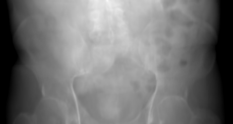
Synthetic MAISI CT. MAISI-v2, rectified flow (rflow-ct), generated with 30 inference steps using NV-Generate-CTMR revision 61c4ec709b84. [36]
The archived 480 × 256 calculation uses 1,000 incident photons per pixel and an illustrative water-equivalent conversion at 80 keV. Scatter, spectral response and detector noise are absent. This is a simulated radiograph, not a patient acquisition.
The radiographic display maps optical depth from 2 to 5.3 to black–white, with the same window for every pose. Pixels outside that interval saturate only in the display. The difference image shows absolute change in expected counts with a fixed asinh scale, where white is 704.5 counts. It does not show the sign of the change.
Translations use 0.5 mm steps about the reference, and rotations use 0.01 rad steps about the fixed sacral pivot. Playback traverses the recorded poses and reverses at the ends. The time per frame is a display choice.
Pose matrices and display metadata ·Calculation provenance · Original numerical checks
A noisy logarithm
With the ideal count model and a known, positive open-beam mean, the ratio is unbiased for . Taking its negative logarithm does not give an unbiased measurement of . Zero counts are an immediate problem:
for any finite . At zero counts the logarithm is undefined. Defining would make its expectation infinite.
At high counts, on observations near a positive mean where a local linear approximation is appropriate,
This approximation excludes zero-count observations. A noisy estimated denominator adds calibration uncertainty as well.
Replacing zero counts by a floor produces a finite array. Both this replacement and adding a pseudocount change the statistical properties of the data.
Compare predicted and observed counts directly. For a realised count , the Poisson negative log likelihood, up to terms independent of , is
This follows by substituting into . It never takes a logarithm of the observed count and remains defined when . Its first two derivatives are
For a zero-count observation, this objective decreases as increases and approaches its infimum only as . Shared image structure or additional information must constrain the estimate. With , the unconstrained single-pixel optimum is , and restricting moves that optimum to zero if .
This likelihood follows from the ideal counting model in section 2.1. An energy-integrating or heavily processed image needs a statistical model for that detector output. The choice of comparison domain is part of section 6.2 on registration objectives.
2.6 Evaluating transmission numerically
In the library outlined in section 1.7, transmission sits between path integration and comparison with the observed image. It converts an array of optical depths into the requested primary-signal quantities and supplies derivatives with respect to its declared active inputs. Here we supply optical depths directly, using slabs and numerical test cases whose answers we can establish independently. Chapter 4 will produce those inputs by integrating through a volume.
The slab cases let us check behaviour near zero attenuation and in nearly opaque paths before we have rays to construct or a volume to sample. We will use the same transmission operation when those inputs come from the renderer.
For a collection of pixels, the deterministic operations are
Compute log transmission directly from . Taking an exponential and then its logarithm introduces rounding error and can fail after underflow. Table 2.3 specifies the input, output and numerical contract for this operation.
| Item | Required meaning or behaviour |
|---|---|
| Optical depth | Finite, non-negative, dimensionless for each pixel. |
| Open-beam mean | Finite, non-negative , with explicit scalar or per-pixel broadcasting. |
| Outputs | Dimensionless , expected count , and log transmission if required. No random sampling. |
| Zero open-beam mean | Return zero expected count. An observed normalised transmission is unavailable for that pixel. |
| Invalid physical input | Report negative optical depth, negative mean or non-finite input, and do not silently clip it into the allowed domain. |
| Numerical policy | State storage and accumulation precision, exponential accuracy mode and any treatment of subnormal values. |
| Derivative meaning | Differentiate the declared deterministic map with acquisition parameters fixed, unless they are explicitly active inputs. |
A non-negative parameterisation may be appropriate when optimising an attenuation field. Hidden clipping inside the forward operation would change the function and introduce its own derivative convention at the clipping boundary.
One operator, several useful outputs
The transmission operator, dpt.transmission.transmit, receives L, the optical-depth array produced by the path integrator. The n0 argument supplies illumination when counts are wanted, and the out_ arguments name the quantities the caller will consume. A count-domain registration objective will use out_counts, and a sensitivity calculation will also need the reverse operation developed below.
Its inputs are contiguous, one-dimensional CUDA arrays with binary32 storage, and the caller flattens the detector image and supplies each destination. Omitting out_T avoids storing a transmission image that the next operation does not need. The removed-primary fraction is a fourth, independently selectable output.
def transmit(
    L: Any,
    n0: Any = None,
    *,
    out_T: Any = None,
    out_counts: Any = None,
    out_log_T: Any = None,
    out_removed: Any = None,
    workspace: TransmissionWorkspace,
    stream: Any = None,
    tape: Any = None,
    validate: bool = True,
) -> None:
    """Evaluate selected deterministic outputs in caller-owned binary32 buffers.

    L is finite, non-negative optical depth. n0 is the declared open-beam
    expectation at the detector. No sampling, clipping or implicit transfer is
    performed. The default checks device contents before writing outputs.
    With validate=False the caller guarantees valid *current* device inputs;
    launches remain asynchronous. Pass tape explicitly to record the custom
    first-order adjoint, and retain original inputs until backward completes.
"""TransmissionSpec fixes the representation of the open beam: a Python scalar, a one-element device array or one device value per pixel. A Python scalar is explicitly rounded to binary32 and treated as fixed. A device array may be declared active when its derivative is required. This prevents an accidental broadcast from silently changing an image-sized calibration problem into a single exposure parameter, or vice versa.
Each output approximates its declared real-valued quantity independently. We do not require machine equality between out_counts and the product of n0 with the rounded out_T, or between out_removed and one minus out_T. Those apparently helpful consistency checks would require the more informative output to inherit the rounding damage of the less informative one. The weak- and strong-attenuation cases below show why. The plots draw recorded CUDA samples in the browser. Move over a curve or use its sample slider to inspect the stored values. The slider selects an existing sample rather than evaluating another optical depth.
Open-beam expectation: 1000000
Transmission T
- CUDA transmission
Numerical details
Expected counts λ
- CUDA expected counts
Numerical details
Log transmission
- CUDA log transmission
Numerical details
Lines join recorded samples. Download exact values.
Weak attenuation
When is small, the fraction removed from the primary beam is
Subtracting an already rounded value of from one can lose most of the significant digits in this small difference. A numerically preferable evaluation is
where evaluates accurately near zero. Similarly, if transmission is supplied through a small decrement , then
CUDA provides the device functions expm1f and log1pf for these expressions. We bind them directly through Warp’s native-function mechanism. The ellipses below are declarations whose bodies are the supplied CUDA strings. They do not invoke Python once per pixel. [31]
@wp.func_native("return -expm1f(-optical_depth);")
def removed_primary(optical_depth: wp.float32) -> wp.float32:
    """Evaluate the decrement directly, without subtracting two near-unities."""
    ...


@wp.func_native("return -log1pf(-decrement);")
def optical_depth_from_decrement(decrement: wp.float32) -> wp.float32:
    """Invert a supplied decrement; the caller requires 0 <= decrement < 1."""
    ...
The inverse takes the decrement itself as its input. If a previous calculation rounded transmission to one and then formed the decrement by subtraction, the lost bits have already gone. log1p has no administrative procedure for requesting their return. Similarly, a decrement rounded to one cannot identify a finite optical depth: the inverse API rejects that endpoint instead of inventing a large finite answer.
Removed-primary fraction
- CUDA removed fraction
- 100-digit reference
- 1 − stored T (binary32)
Numerical details
The reference curve is rounded to binary64. 1 − stored T (binary32): 58 stored zeros, first sampled zero at Optical depth L = 9.99999996e-13. Zeros appear on a separate labelled rail, outside the logarithmic scale.
Inverse error (binary32 ULPs)
- CUDA inverse error
Numerical details
Error against an independent high-precision inverse.
Lines join recorded samples. Download exact values.
The removed-primary fraction includes photons that scattered out of the uncollided history. It is not an absorbed-energy fraction or a dose estimate.
Strong attenuation
For large , the exponential can underflow to zero even while optical depth and log transmission remain representable. Keeping log transmission allows comparisons in that domain without introducing a tiny transmission floor.
An absolute error of is excellent for a transmission near one and disastrous for a transmission near . A validation criterion must say which regime it covers. Relative error is useful for positive, representable reference values, while behaviour near underflow needs a separate check. The underflow threshold depends on the numeric type, treatment of subnormal values and mathematical implementation.
Storage precision and intermediate precision need separate decisions. Consider the mathematical stress input with an open-beam mean near . Transmission is below the binary32 subnormal range, but the expected count is approximately and remains representable. Multiplying the open beam by a transmission value already stored as zero destroys that count. This is a test of numerical range, not a claim about a plausible clinical exposure.
Our arrays remain binary32. The kernel keeps the exponential factor in a binary64 register until the requested products have been formed, then rounds each output independently. For , it evaluates the ordinary binary32 exponential and promotes the result. Above that cutover it evaluates the exponential in binary64 from the exactly promoted input. At the cutover the binary32 exponential is still normal: promotion preserves its available precision, while the wider exponent range protects later products. The value 64 is an implementation boundary, with neighbouring representable inputs tested on both sides, and it has no physical significance.
@wp.func_native("return -value;")
def log_transmission_exact(value: wp.float32) -> wp.float32:
    """Use IEEE unary negation; Warp 1.17's generic neg is ``0 - value``."""
    ...


@wp.func
def transmission_factor(optical_depth: wp.float32) -> wp.float64:
    """Keep exponent range until all requested physical products are formed."""
    if optical_depth <= wp.float32(64.0):
        # Here exp(-L) is normal in FP32. Promotion retains its range, while
        # keeping the common case on the single-precision exponential path.
        return wp.float64(wp.exp(-optical_depth))
    return wp.exp(-wp.float64(optical_depth))
The kernel forms count directly from factor. The wider temporary lives within the kernel, so there is no hidden binary64 image to allocate, write and reread. Log transmission takes a different path altogether: unary negation of the input, preserving the sign of zero as well as every finite magnitude. It does not depend on the exponential’s range.
Stored transmission T
- CUDA transmission
Numerical details
Numerical stress test with an open-beam expectation of 1.00000002e+30. CUDA transmission: 103 stored zeros, first sampled zero at Optical depth L = 104.375. Zeros appear on a separate labelled rail, outside the logarithmic scale.
Stored expected counts λ
- CUDA expected counts
Numerical details
Numerical stress test with an open-beam expectation of 1.00000002e+30. CUDA expected counts: 29 stored zeros, first sampled zero at Optical depth L = 173.75. Zeros appear on a separate labelled rail, outside the logarithmic scale.
Lines join recorded samples. Download exact values.
The kernel disables fast mathematics and permits fused multiply-add contraction. FMA rounds a multiply-add once, whereas separate instructions round its product first. Flush-to-zero and approximate intrinsics are different choices that can change the small-value behaviour. NVIDIA’s floating-point guide describes those distinctions. Our tests cover the selected settings rather than assuming that the word CUDA guarantees a particular elementary-function accuracy. [32]
Fusing the work that is actually requested
Each CUDA thread handles one pixel, computing and writing only the outputs the caller requests. Those choices are fixed in the output mask when the kernel specialisation is created, allowing wp.static to remove the unused branches at compile time. A counts-only call therefore leaves transmission unstored and skips log transmission; a log-only call skips the exponential altogether. Array length and illumination values, by contrast, remain runtime inputs: changing the exposure does not require recompilation.
@cache
def get_forward_kernel(mask: int, beam_mode: int):
    """Return a specialised pointwise kernel, launched with ``dim=P``.

    Inputs: L, beam_array, beam_scalar. Outputs: T, counts, log_T, removed.
    Static selection eliminates unused array reads, stores and mathematics.
    """
    if mask < 1 or mask > 15 or beam_mode not in (0, 1, 2, 3):
        raise ValueError("Invalid output mask or beam mode")
    if mask & 2 and beam_mode == 0:
        raise ValueError("Counts require an open beam")

    @wp.kernel(module="unique", module_options=STRICT_OPTIONS)
    def forward(
        optical_depth: wp.array(dtype=wp.float32),
        beam: wp.array(dtype=wp.float32),
        beam_scalar: wp.float32,
        transmission: wp.array(dtype=wp.float32),
        counts: wp.array(dtype=wp.float32),
        log_transmission: wp.array(dtype=wp.float32),
        removed: wp.array(dtype=wp.float32),
    ):
        p = wp.tid()
        depth = optical_depth[p]
        if wp.static(mask & 3 != 0):
            factor = transmission_factor(depth)
            if wp.static(mask & 1 != 0):
                transmission[p] = wp.float32(factor)
            if wp.static(mask & 2 != 0):
                illumination = beam_scalar
                if wp.static(beam_mode == 2):
                    illumination = beam[0]
                elif wp.static(beam_mode == 3):
                    illumination = beam[p]
                # In particular, never multiply illumination by stored T.
                count = wp.float32(wp.float64(illumination) * factor)
                if count == wp.float32(0.0):
                    count = wp.float32(0.0)
                counts[p] = count
        if wp.static(mask & 4 != 0):
            log_transmission[p] = log_transmission_exact(depth)
        if wp.static(mask & 8 != 0):
            decrement = removed_primary(depth)
            if decrement == wp.float32(0.0):
                decrement = wp.float32(0.0)
            removed[p] = decrement

    return forward
This fusion saves launches and repeated image traffic, neither of which is desirable if we want matters to proceed at pace. With a per-pixel beam and all four outputs, the pointwise forward operation requests two binary32 reads and four writes: 24 bytes per pixel before cache effects and transaction overhead. A transmission-only call needs one read and one write, or 8 bytes per pixel. These are traffic counts from the source, not measured DRAM bandwidth. Validation scans and scalar reductions have their own traffic and must be accounted for separately.
We also avoid adding shared-memory staging to a pointwise calculation with no cross-pixel reuse. It would introduce storage and synchronisation without reducing the compulsory image reads. The branch at the precision cutover is different: pixels can take different arithmetic paths, so mixed ordinary and extreme inputs belong in profiling workloads. We check the numerical results and repeat the device measurements after changing either arithmetic path.
Differentiating with respect to optical depth and the open-beam mean gives
At fixed open-beam mean and positive , a small optical-depth change changes the expected count by approximately . Under the ideal Poisson model, the count standard deviation is , so the size of that predicted change relative to the counting fluctuations is approximately . This ratio shrinks as attenuation increases, consistent with the falling Poisson curvature . Rescaling the objective can enlarge its numerical gradients, but it does not improve this local signal-to-noise ratio.
A backward pass that preserves the same range
An optimiser rarely asks for an isolated derivative at one pixel. It supplies a cotangent for each requested output: the derivative of its scalar objective with respect to that output. Write these incoming weights as , , and for transmission, counts, log transmission and removed fraction. The optical-depth contribution is . This is a vector–Jacobian product (VJP): it combines the objective’s weights with the local derivatives without ever constructing a dense Jacobian.
@wp.func
def weighted_depth_adjoint(
    factor: wp.float64,
    illumination: wp.float32,
    seed_transmission: wp.float32,
    seed_counts: wp.float32,
    seed_log: wp.float32,
    seed_removed: wp.float32,
) -> wp.float64:
    """Differentiate the real-valued map, retaining range before rounding."""
    optical = (wp.float64(seed_removed) - wp.float64(seed_transmission)) * factor
    count = wp.float64(seed_counts) * wp.float64(illumination) * factor
    return optical - count - wp.float64(seed_log)
The derivative is that of the declared smooth real-valued map, evaluated approximately at the supplied floating-point inputs. It is not the derivative of a staircase of rounded storage values. Differentiating that staircase would produce zero almost everywhere and be singular at its jumps, which is a poor basis for moving a bone into place.
Reusing rounded forward outputs is especially dangerous here. A large incoming weight can make representable even when stored transmission is zero. A small open-beam mean and a large count cotangent can similarly produce a useful product after stored counts have underflowed. For removed fraction, 1 - stored_removed can already be zero. The VJP therefore recomputes the factor from the original optical depth and forms weighted products in binary64 registers. It also computes the open-beam derivative directly: dividing counts by the open beam would fail at the perfectly valid input .
There is one local open-beam derivative per pixel when the beam is an active image. When the active beam is a single shared device value, its gradient instead sums over all pixels. The implementation forms binary64 partial sums in tiles of 256 pixels and reduces those partials through a fixed tree. The tree allocation, later reduction levels and final cast use the shared reduction code also used by projection and objectives, while the first stage retains this operator’s range-sensitive products. This avoids sending every thread to contend for the same global scalar. It also avoids retaining a full-sized array of binary64 contributions: only the much smaller tree of partials is persistent. A separate reduction pass rereads optical depth and count cotangents. That cost is explicit, and the reduction must finish before its scalar result can be used.
@cache
def get_beam_partial_kernel():
    """Inputs L, seed_counts; output FP64 partials.

    Use ``launch_tiled(dim=ceil(P/256), block_dim=256)``. Tile loads zero-pad
    their bounds, so padded seeds contribute zero even though exp(-0) is one.
    The separate pass deliberately avoids retaining an 8P-byte contribution
    image or contending for a global scalar. Its traffic is accounted separately.
    """

    @wp.kernel(module="unique", module_options=STRICT_OPTIONS)
    def partials(
        optical_depth: wp.array(dtype=wp.float32),
        seed_counts: wp.array(dtype=wp.float32),
        output: wp.array(dtype=wp.float64),
    ):
        block = wp.tid()
        depths = wp.tile_load(optical_depth, shape=TILE_SIZE, offset=block * TILE_SIZE)
        seeds = wp.tile_load(seed_counts, shape=TILE_SIZE, offset=block * TILE_SIZE)
        contributions = wp.tile_map(beam_contribution, depths, seeds)
        total = wp.tile_sum(contributions)
        wp.tile_store(output, total, offset=block)

    return partials
The inverse helper follows the same rule: its VJP uses the original decrement and evaluates . As approaches one, this derivative grows. That is the inverse problem’s conditioning, not an invitation to clamp the denominator. A final gradient that cannot be represented in binary32 sets a numerical error flag, and the checked completion boundary raises GradientRangeError. A legitimate forward underflow and an unusable overflowing gradient are different outcomes.
Owning storage, streams and reverse execution
prepare_transmission binds a workspace to one CUDA stream and allocates its persistent diagnostics and any required scalar-reduction scratch. The caller allocates inputs, destinations and, for taped execution, gradient buffers. These buffers must remain alive until the stream has finished using them. Original inputs must also remain unmodified until backward completes, because recomputation deliberately reads them again. Two concurrent operations need separate workspaces or explicit serialisation: sharing an object in Python does not order GPU execution.
The default checked call validates shape, dtype, device, capacity and actual memory-range overlap, then scans device values before launching numerical writes. It rejects unsupported layouts, so the caller must explicitly prepare contiguous inputs. An invalid depth is still invalid when illumination is zero: multiplying it by zero would conceal an upstream error. Failure diagnosis may copy the offending input back to identify its index, while a successful checked call only needs the small status result on the host.
Inside a composition whose current inputs are already guaranteed valid, validate=False omits the content scan and its synchronisation. Metadata checks remain. This boundary is useful for a warmed CUDA graph or a device-resident optimisation loop, but it transfers responsibility for the current values to the caller. Mutating an array after checking it does not preserve a certificate of good behaviour. Compilation and allocation must happen before graph capture, and graph replay then reuses the same buffers and launch structure.
Passing a tape explicitly records the library’s custom first-order backward callback through Warp’s Tape.record_func. Warp provides this hook for custom reverse work and tracks the participating arrays, while our adapter supplies the VJP and its buffer-consumption rules. [33] A shared input can influence the objective through several downstream operations, so its cotangent must add their contributions rather than overwrite an earlier one. Our adapter therefore accumulates input cotangents. It consumes ordinary output cotangents after all local contributions have been read, while explicitly retained gradients remain available. Before an independent reverse pass, tape.zero() clears the previous derivative sums so they are not included in the new calculation.
After backward, workspace.check_status() waits for the owning stream and reports gradient-range failure before the optimiser accepts the result.
Cross-stream producers and consumers require explicit events and waits. Internal stream scopes disable Warp’s automatic entry synchronisation: once ownership is established, inserting another event and wait into every call would add ordering work without supplying a missing dependency.
A VJP recorded on an enclosing tape is rejected: this operator supports first derivatives, and silently returning zero for a second derivative would be an especially unhelpful form of optimism.
Supporting second derivatives would require another defined and independently verified differentiation boundary. Chapter 5 develops the broader derivative execution problem once transmission is composed with geometry and integration.
2.7 Checks before adding geometry
The transmission law gives us reference cases whose answers can be derived independently of a renderer. Table 2.4 pairs each case with a common footgun in modelling transmission.
| Case | Reference result | What it can detect |
|---|---|---|
| Empty path or zero attenuation | , , | Incorrect initial values or path handling. |
| Homogeneous segment | , | Unit errors and an incorrect exponent sign. |
| Split a homogeneous segment | when | Segment weights that fail to preserve length. |
| Fixed layered path | Incorrect material association or missing segments. | |
| Convert the length unit | Coefficients and distances expressed in different units. | |
| Add a non-negative segment | Sign mistakes or unphysical numerical behaviour. | |
| Finite zero-attenuation derivative | at | A backward rule that incorrectly vanishes in an empty path. |
A varying coefficient adds a check that a constant slab cannot provide. Prescribe
with in inverse length, in inverse length squared, and coefficients chosen so that throughout the interval. Direct integration gives
Evaluate the polynomial antiderivative from the specified parameters to obtain an independent reference for the sampled path integral. Calling the same quadrature through another wrapper would repeat its errors.
Derivative checks can use the closed-form slab sensitivities from section 2.3. For a positive interior optical depth and a step satisfying , compare the analytic derivative with the central difference
For this smooth function, truncation error decreases quadratically with until floating-point effects become significant. Check a range of steps. At the boundary , a centred perturbation would leave the physical input domain, so use a suitable one-sided check or explicitly test an agreed mathematical extension.
An oracle that does not repeat the kernel
The test reference converts each supplied binary32 value into its exact decimal value before evaluating the mathematics at high precision. Comparing a GPU input rounded from a decimal literal with the unrounded literal would charge input quantisation to the kernel. The reference uses independent scalar Decimal expressions and explicit binary32 rounding, and it never calls the CUDA helper to obtain the expected answer. Increasing reference precision checks that the oracle itself has settled.
def analytic_cases() -> tuple[AnalyticCase, ...]:
    """Closed-form path cases, without claiming to validate a path integrator.

    All coefficients and lengths below are exact dyadic mathematical stress inputs.
    The mm and cm expressions describe the same optical depth in different units.
    """
    coefficient, distance = Decimal("0.125"), Decimal(4)
    first_length, second_length = Decimal(1), Decimal(3)
    intercept, slope = Decimal("0.125"), Decimal("0.0625")
    return (
        AnalyticCase("empty", Decimal(0), "empty path"),
        AnalyticCase("zero-attenuation", Decimal(0), "mu = 0"),
        AnalyticCase("homogeneous", coefficient * distance, "mu*d"),
        AnalyticCase(
            "split-homogeneous",
            coefficient * first_length + coefficient * second_length,
            "mu*d1 + mu*d2",
        ),
        AnalyticCase("layered", Decimal("0.25") * 2 + Decimal("0.5") * 3, "mu1*d1 + mu2*d2"),
        AnalyticCase("millimetres", Decimal("0.125") * 4, "0.125/mm * 4 mm"),
        AnalyticCase("centimetres", Decimal("1.25") * Decimal("0.4"), "1.25/cm * 0.4 cm"),
        AnalyticCase(
            "added-segment",
            coefficient * distance + Decimal("0.25"),
            "mu*d + non-negative optical depth",
        ),
        AnalyticCase(
            "linear-coefficient",
            intercept * distance + slope * distance * distance / 2,
            "integral_0^d (a+b*s) ds",
        ),
    )
These fixtures validate transmission at known optical depths. The ray integrator must independently recover those depths from the geometry and material field.
For normal outputs, the value tests use a budget of four binary32 units in the last place (ULPs) for transmission, removed fraction and the inverse, and eight for expected counts. A ULP measures spacing between neighbouring representable values at the result’s magnitude. Subnormal results have their own one-ULP budget, and exact cases such as log negation are checked directly. The budgets are acceptance criteria, not statements that every value reaches the limit. Each independently requested output is compared with its own correctly rounded reference.
VJPs need a different error scale. Two large weighted contributions can nearly cancel, leaving a small correct gradient. Dividing the error by that residual would make the apparent relative error arbitrarily large. We instead scale the acceptance bound by the magnitudes of the contributing terms, with explicit rounding allowances, and scalar beam gradients also account for the reduction depth. The tests include cancellation, zero illumination, extreme weights and subnormal inputs.
def directional_check(
    evaluate: Callable[[float], float],
    anchor: float,
    analytic_derivative: float,
    *,
    exponents: Iterable[int] = range(2, 25),
) -> tuple[DirectionalRecord, ...]:
    """Sweep a real operator callback over admissible, distinct binary32 inputs.

    Interior anchors use centred differences; zero uses a second-order one-sided
    stencil. No convergence claim is inferred from the smallest step: callers retain
    all records to expose truncation, agreement and storage-rounding regimes.
    """
    centre = binary32(anchor)
    if centre < 0:
        raise ValueError("anchor must be non-negative")
    records: list[DirectionalRecord] = []
    for exponent in exponents:
        step = 2.0**-exponent
        right = binary32(centre + step)
        if right == centre:
            continue
        if centre == 0:
            second = binary32(2 * step)
            if second <= right:
                continue
            derivative = (-3 * evaluate(centre) + 4 * evaluate(right) - evaluate(second)) / (
                2 * right
            )
            stencil = "one-sided-second-order"
        else:
            if centre - step < 0:
                continue
            left = binary32(centre - step)
            if left == centre or centre - left != right - centre:
                continue
            derivative = (evaluate(right) - evaluate(left)) / (right - left)
            stencil = "centred"
        records.append(
            DirectionalRecord(
                right - centre, derivative, abs(derivative - analytic_derivative), stencil
            )
        )
    return tuple(records)
The finite-difference helper accepts a callback to the actual GPU operator. It checks that perturbed inputs remain distinct after binary32 rounding and retains every admissible step. At an interior point, agreement should improve over a range of steps before storage rounding dominates, while at zero, the helper uses a second-order one-sided stencil. Selecting only the smallest step would often select the least informative comparison. Agreement with both the independent analytic VJP and the directional sweep checks different failure modes.
Execution is part of correctness
A formula test cannot detect every GPU integration error. We therefore also need empty batches, lengths that leave a partial tile, and a scalar reduction large enough to require several levels. Reusing a large workspace for a smaller batch must not include stale partial sums. Output masks, fixed and active beam representations, overlapping array views, non-default streams and graph replay each exercise a distinct part of the contract. Tape tests compose transmission with surrounding kernels so that missing contributions or incorrectly consumed cotangents become observable.
Device timing begins after compilation and warm-up. Checked-call timing includes the validation scan and status synchronisation, while CUDA-event batches measure the warmed stream interval, including gaps while the host submits work. Isolated per-kernel durations come from the profiler. Forward and backward measurements record requested outputs, pixel count, beam representation, precision settings, scratch size and launch structure. A short runtime without that context cannot tell us whether an optimisation removed work, hid a transfer or simply measured a smaller problem. Memory and synchronisation tools complement numerical tests, but a clean run in either category does not replace the other.
def evaluate_sweep(wp: Any, np: Any, depths: Any, beam: float, device: Any) -> dict[str, Any]:
    """Execute all four canonical outputs, then check every stored value."""
    workspace = prepare_transmission(
        TransmissionSpec(beam="scalar"), device=str(device), max_pixels=len(depths)
    )
    optical_depth = wp.array(depths, dtype=wp.float32, device=device)
    outputs = [wp.empty(len(depths), dtype=wp.float32, device=device) for _ in OUTPUT_NAMES]
    transmit(
        optical_depth,
        beam,
        workspace=workspace,
        **dict(zip(OUTPUT_ARGUMENTS, outputs, strict=True)),
    )
    wp.synchronize_stream(workspace.stream)
    measured = [output.numpy() for output in outputs]
    cases: list[dict[str, Any]] = []
    for index, depth in enumerate(depths):
        reference = forward_reference(float(depth), beam)
        checks = {}
        for name, values in zip(OUTPUT_NAMES, measured, strict=True):
            result = value_error(
                float(values[index]), getattr(reference, name), counts=name == "counts"
            )
            exact_log = name != "log_T" or struct.pack("!f", float(values[index])) == struct.pack(
                "!f", -float(depth)
            )
            checks[name] = {
                "actual": float(values[index]),
                "reference_decimal": str(getattr(reference, name)),
                "ulps": result.ulps,
                "allowed_ulps": 0 if name == "log_T" else result.allowed_ulps,
                "passed": result.passed and exact_log,
            }
            if not result.passed or not exact_log:
                raise AssertionError(f"{name} failed at optical depth {depth}: {checks[name]}")
        cases.append({"optical_depth": float(depth), "checks": checks})
    return {
        "beam": float(np.float32(beam)),
        "cases": cases,
        "outputs": {
            name: values.tolist() for name, values in zip(OUTPUT_NAMES, measured, strict=True)
        },
        "optical_depths": depths.tolist(),
    }
To form an image, every detector pixel needs the correct path through the object. Chapter 3 fixes the coordinate conventions for those paths and for moving the object while leaving its material attenuation coefficients unchanged.
References
- Dance, D. R., Christofides, S., Maidment, A. D. A., McLean, I. D. and Ng, K.-H. (eds.) (2014). Diagnostic Radiology Physics: A Handbook for Teachers and Students. Vienna: International Atomic Energy Agency. https://www.iaea.org/publications/8841/diagnostic-radiology-physics
- Hubbell, J. H. and Seltzer, S. M. (1995). Tables of X-Ray Mass Attenuation Coefficients and Mass Energy-Absorption Coefficients 1 keV to 20 MeV for Elements Z = 1 to 92 and 48 Additional Substances of Dosimetric Interest. Gaithersburg, Maryland: National Institute of Standards and Technology. https://doi.org/10.6028/NIST.IR.5632
- Gopalakrishnan, Vivek and Golland, Polina (2023). Fast Auto-differentiable Digitally Reconstructed Radiographs for Solving Inverse Problems in Intraoperative Imaging. Clinical Image-Based Procedures, 13746, 1-11. Cham: Springer. https://doi.org/10.1007/978-3-031-23179-7_1
- NVIDIA Corporation (n.d.). CUDA Math API Reference Manual 13.0: Single Precision Mathematical Functions. https://docs.nvidia.com/cuda/archive/13.0.0/cuda-math-api/cuda_math_api/group__CUDA__MATH__SINGLE.html
- Whitehead, Nathan and Fit-Florea, Alex (n.d.). Floating Point and IEEE 754. NVIDIA Corporation. https://docs.nvidia.com/cuda/archive/13.0.0/floating-point/index.html
- NVIDIA Warp contributors (n.d.). Warp 1.17.0: Tape implementation. https://github.com/NVIDIA/warp/blob/v1.17.0/warp/_src/tape.py