Registering a CT volume to calibrated radiographs
A known CT volume and calibrated X-rays give us a concrete registration problem. We put pose recovery to work across views and assess the recovered geometry independently of the image fit.
The CT tells us where a structure was when the volume was acquired. The radiograph tells us where its projected attenuation appears now. Registration estimates the rigid transform connecting those two descriptions. Once that transform is known, a point selected in the volume can be located in the imaging system and projected into each calibrated view. A convincing overlay is useful, but it will have to earn its keep as evidence of geometric recovery.
Chapter 6 established the pose chart, image derivatives and optimiser. Here we assemble an application around them: supplied data with documented units, several views that must agree on one pose, and evaluation information withheld from the fit. The executable example is python/dpt/examples/registration.py. It fits calibrated primary photon counts with a fixed volume and fixed acquisition geometry. More general image comparisons and mismatch models have a place in the study, but require the corresponding measurement operators.
Our worked example starts with the supplied CT-ORG case 2 volume and generates two calibrated, orthogonal radiographs. From the identity transform, it recovers the shared pose in 16 accepted updates and reduces RMS target error from 3.77 mm to 0.010 mm. It also reaches the numerical stopping tolerance and predicts two reserved views accurately. The complete recipe includes the prepared input, its provenance and one driver connecting generation, fitting and independent evaluation. The anatomy comes from acquired CT; its 80 keV attenuation assignment and the photon-count radiographs are simulated.
11.1 Define the registration case
The case begins with an attenuation field , expressed in object coordinates, and a set of radiographs acquired with known source and detector geometry in a shared world frame. Let map object points into world coordinates. For a physical target point and calibrated projection map of view ,
Homogeneous coordinates are implicit in the transform product. This convention fixes what the reported transform means: its translation is expressed in world millimetres, and its rotation acts on object-frame column vectors. A camera-pose estimate from another package may encode the inverse map. Compare the action on physical points before comparing twelve numbers printed by two libraries.
The volume array has shape , with x varying fastest. GridSpec supplies spacing in order, the first sample-centre position, and a right-handed orientation matrix. Attenuation is in inverse millimetres. CT numbers are not that attenuation field without a declared conversion, and a polychromatic CT reconstruction does not automatically provide a monochromatic material map. Preserve the conversion recipe and its calibration source alongside the original volume. Chapter 4 describes the interpolation and finite-support assumptions that the projector will actually use.
Each detector specifies shape , its first pixel centre, column and row basis vectors, and their physical pitches. Distortion correction, cropping or resampling changes how image indices map to rays. The geometry must describe the array passed to the objective, including any updated origin and spacing. Image orientation guesses are expensive when the optimiser takes them seriously.
A registration case also needs a physical claim about rigidity. A single bone can often be treated as one rigid object for a specified acquisition interval, but neighbouring anatomy may violate that assumption. Removing a neighbouring structure from the volume does not remove its attenuation from the radiograph. Define the region whose agreement will be tested and explain how unmodelled material along those same rays is handled. Figure 11.1 shows the coordinate frames and the shared unknown pose.
One representative calibrated view
The field and sampling grid move together with O.
Attenuation in mm⁻¹, with spacing and origin in mm.
Source position, detector pixel centres and open-beam counts, with calibrated detector axes and pitches.
11.2 Compare compatible image quantities
The example assumes independent photon counts with a spatially uniform, calibrated open-beam expectation in each view. The primary prediction is
The integration follows the finite source-to-pixel segment in world coordinates. Rigid motion preserves length, so the object-frame integrator retains millimetres along that segment. Exposure belongs to the view, while the attenuation volume and the object pose are shared.
For observed counts and a fixed binary inclusion mask , the implemented objective is a sum of Poisson half-deviances:
For , the limiting expression is . For positive , a zero predicted mean is invalid. The half-deviance differs from the negative log-likelihood by an observation-only constant, so both give the same pose gradient. With positive predicted means, differentiation in any smooth pose coordinate gives
The FP64 primary composition forms the weighted depth cotangent directly; the projection VJP then pulls it back to pose. The example uses reduction="sum", preserving the likelihood contribution of every included observation. Dividing each view by its own pixel count would define a different relative weighting. If exposures differ, their count statistics already enter through . Assigning each image the same arbitrary scale would erase part of that model.
A binary mask excludes specified pixels from the sum. Fix it before the solve and retain it with the input record. Excluding bad detector elements is defensible when their identity is independently known. Excluding whatever disagrees with the current pose changes the objective and can conceal the anatomy that would disprove the fit. Saturation also needs a declared treatment: the stored ceiling is not an ordinary unsaturated Poisson count. The example accepts finite integer-valued FP32 observations through . Every excluded pixel must contain zero in the supplied preprocessed observation, so an underflowed prediction there cannot invalidate the count calculation before the mask is applied. Those zeros are excluded placeholders. Preserve the raw source and record the preprocessing recipe with the supplied array’s provenance.
Most energy-integrating or processed fluoroscopy images need a different comparison. Dark subtraction and flat-field division generally destroy the raw-integer-count interpretation. A log-transmission objective must use consistently, while conventional positive log projections use the opposite sign. Where a display pipeline cannot be inverted, correlation or gradient-based similarity can still define a registration criterion, without acquiring a measurement likelihood by wishful notation. Otake and colleagues used normalised gradient information with multistart optimisation to address deformation and content mismatch in spine registration. [18] Figure 11.2 follows the two supplied count images from the initial pose to the recovered one. Its logarithmic window makes the attenuated anatomy visible; the optimiser still compares counts through the half-deviance above. The gradient history and independent target errors show why the fitted images deserve more confidence than an overlay alone.
Loading recorded arrays…
Initial prediction
Observed counts
Recovered prediction
Display and array data
Both views retain all 128 × 128 detector samples. The same logarithmic count window is used for each panel; displayed pixels are not smoothed.
Reaching the stopping criterion
- Accepted pose
- Required ≤ 0.001
Recovering the generating pose
- Independent evaluation
The optimiser sees the two count images, the known volume and fixed calibration. After fixing the result, the evaluator compares its action on the eight target points with their generating positions. The final gradient and target error answer different questions, and both pass.
| Quantity | Result | Criterion |
|---|---|---|
| Solver termination | Gradient tolerance; 16 accepted updates | Scaled gradient ≤ 0.001 |
| Final scaled gradient | 0.000119134 | ≤ 0.001 |
| RMS target error | 3.769 → 0.00998 mm | ≤ 1 mm |
| Worst target error | 0.01220 mm | ≤ 2 mm |
| Reserved-view mean error | 0.00448 Poisson SD RMS | ≤ 1 Poisson SD RMS in both views |
Reproduction and recorded data
11.3 Initialise within a defensible search region
An initial pose can come from tracked geometry, independently acquired landmarks, or an explicitly trained proposal method. Record what information produced it. A pose obtained by perturbing the reference transform is a controlled capture-range experiment, and it is not an initialisation procedure available on a new acquisition without that reference.
The example anchors one PoseChart at the supplied initial transform . Its dimensionless coordinates define
The first three scales have units of millimetres and the last three radians. The hat maps the scaled six-vector into . A rotation scale should reflect the lever arm of the anatomy being fitted: for a point at distance from the object origin, a small angle produces displacement of order . This relationship gives translation and rotation steps comparable physical meaning without pretending that millimetres and radians are interchangeable.
The anchor and scales remain fixed during a solve. Away from the anchor, the projector’s derivative for a fresh local right increment must be pulled back through the right Jacobian of the exponential before it becomes a derivative in . PoseChart.gradient() performs that calculation. Simply rescaling six local derivatives is insufficient at a general trial pose. The declared rotation radius also bounds the chart, and crossing it requires a new solve with cleared optimiser history.
The driver starts at and performs one local solve. For multistart registration, give each starting pose its own chart and reuse the same fixed observations. Choose the result without consulting the evaluation reference. Charge every proposal its full evaluation cost. Coarse-to-fine registration similarly needs a documented physical image pyramid, with geometry and comparison updated at every level. Blurring counts and retaining the independent Poisson interpretation is generally inconsistent.
DiffPose provides a concrete alternative initialisation strategy: a patient-specific network learns pose from rendered projections of the known CT, then differentiable image optimisation refines its prediction. [23] Its relevance here is the separation between a proposal mechanism and local refinement. Adopting that approach would require its own training record and evaluation of acquisition mismatch, as well as the local solver’s tests.
11.4 Add views to constrain the same pose
With simultaneous views, or sequential acquisitions during which the object remains still, every view evaluates the same . Each source and detector can occupy a different position in the common world frame. One view’s almost invisible depth motion may then become a conspicuous lateral motion in another. That benefit depends on the object and field of view as well as angular separation.
The implementation gives each view its own prepared evaluator, all holding the same PoseChart object. Each evaluator returns six derivatives already expressed in that chart. The host sums those small results:
class SharedPoseObjective:
    """Sum views in one immutable chart; each evaluator owns its image scratch."""

    def __init__(self, views: tuple[PreparedView, ...], chart: PoseChart) -> None:
        if not views or any(view.evaluator.chart is not chart for view in views):
            raise ContractError("all views must share the same PoseChart object")
        self.views, self.chart = views, chart

    def __call__(self, parameters: Vector) -> Evaluation:
        values = tuple(view.evaluator(parameters) for view in self.views)
        return Evaluation(
            math.fsum(value.loss for value in values),
            tuple(math.fsum(value.gradient[k] for value in values) for k in range(6)),
        )
Averaging transforms fitted independently to each view does not minimise this joint objective. Gradients must also use the same frame and scales before they can be added. Requiring one chart object keeps the anchor and scales identical in every view.
A local information calculation explains the geometric benefit. Write at a declared pose. Under the positive-mean independent Poisson model, the expected information is
For any direction , its quadratic form is a sum of nonnegative squared directional sensitivities. Adding an independent view cannot reduce this information matrix in positive-semidefinite order under the stated fixed model. It can still leave a common null direction unresolved. Nearly repeated views may improve precision where information already exists while contributing little to the weakest direction.
Local curvature says nothing about a distant pose producing another plausible projection. A repeated anatomical pattern can admit competing solutions even where the neighbourhood of each solution is well conditioned. Likewise, if the object moves between exposures, one shared pose no longer describes the acquisition. Fit time-specific poses or account for motion before interpreting a sharper local minimum as stronger evidence. The worked case uses two full orthogonal views so that the reader can first complete this shared-pose recovery. The restricted-view example at the end of the chapter then shows what happens when that information is removed.
11.5 Account for imperfect agreement
A primary renderer fitted to measured data will often leave structured residuals. Miscalibrated geometry can shift edges across the image. Scatter can add a smooth component. Anatomical change can create a disagreement confined to one region but impossible for a single rigid transform to repair. Inspecting residuals by view and location helps distinguish these explanations, while the total objective hides that structure.
Allowing a nuisance parameter changes what the images can determine about pose. Take a positive-semidefinite joint information matrix for , including any justified prior, and assume its nuisance block is positive definite. Eliminating those locally identifiable nuisance directions gives
The inverse requires a nonsingular nuisance block, possibly after a justified prior has been included. Directions that can be explained by either pose or nuisance variation lose pose information. For example, unconstrained source motion can imitate changes in the object’s position relative to that source. A numerical optimiser cannot distinguish parameter names that produce the same measurements.
The supplied-count driver therefore keeps geometry and open-beam counts fixed. It does not estimate scatter, detector offsets or spectral parameters. Where calibrated spectral data and a material representation are available, SpectralPoseEvaluator provides the canonical multiview and shared-nuisance composition discussed in §7.6. Its identified gain/exposure convention still matters: two unrestricted multiplicative scales cannot be recovered separately from their product.
A mismatch study should begin with a separately checked matched-model reference, then change one declared factor at a time. Keep the supplied anatomy and image evidence traceable through every variant. For real acquisitions, residual patterns can motivate a model revision, but cannot by themselves establish which physical mechanism caused the error. A rigid optimiser cannot repair an incorrect anatomical model by becoming more enthusiastic.
11.6 Assemble the complete application
The supplied-input JSON case declares its input arrays by name, with file paths, SHA-256 digests, source descriptions, redistribution rights and units. The application section supplies the grid and chart, a positive ray-sample count, the recovery policy and calibrated views. The accompanying python/dpt/examples/README.md describes the complete input contract and the command for running the example. The worked recipe supplies a prepared, attributed input and writes new observations and execution records to a separate output directory. Its orchestration driver generates those observations before calling the supplied-count fitter; the fitter itself receives only the declared arrays and calibration.
Preparation validates the supplied arrays and uploads the attenuation field once. Each view retains its own observations and binary mask, while sharing that attenuation allocation and a CUDA stream. The source below connects those persistent inputs to the existing projection, transmission and objective operators:
                    problem = PrimaryPoseProblem(
                        grid=grid,
                        geometry=geometry,
                        attenuation=attenuation,
                        observation=wp.array(observed.reshape(-1), dtype=wp.float32, device=device),
                        objective=ObjectiveSpec(
                            kind="poisson", domain="counts", reduction="sum", weighted=True
                        ),
                        open_beam=beam,
                        weights=wp.array(mask.reshape(-1), dtype=wp.float32, device=device),
                        samples_per_ray=samples,
                        precision=configuration.get("precision", "float64"),
                        integration=configuration.get("integration", "midpoint"),
                    )
evaluator = PrimaryPoseEvaluator(problem, chart, device=device, stream=stream)Image-sized intermediate arrays remain on the device throughout optimisation. The host exchanges rigid-transform values, a scalar objective and six derivatives with the device, together with numerical-status checks. Summing those derivatives on the host does not require copying the detector images. The example evaluates views sequentially on its shared stream.
The optimiser needs one callback and one initial six-vector. Its policy records evaluation and iteration budgets separately, together with stopping tolerances. The returned state is the last accepted state:
        initial: Vector = (0.0,) * 6
        result = recover_parameters(objective, initial, policy=policy)
        recovered = chart.pose(result.parameters)
        run.write_json(
            "optimisation.json",
            {
                "pose_object_to_world": asdict(recovered),
                "chart": asdict(chart),
                "policy": asdict(policy),
                "precision": views[0].evaluator.problem.precision,
                "integration": views[0].evaluator.problem.integration,
                "result": asdict(result),
                "stationary": result.stationary,
            },
)A gradient-tolerance stop records numerical stationarity in this chart. A small step or loss change records stagnation. Neither establishes geometric success. Preserve line-search failures and exhausted budgets in the study record rather than excluding inconvenient runs after looking at their images.
One final evaluation per view is deliberately outside the solver budget. Reused prediction scratch may contain a rejected trial, so the example recomputes every view at the accepted pose before exporting its count prediction. Those export evaluations are counted separately in fit-report.json. Multiplying solver calls by the number of views gives a reported upper bound on view evaluations: a rejected numerical trial can stop before all views are evaluated. The report also retains each view’s half-deviance and included-pixel count.
Near the solution, rounding intermediate counts can obscure the small loss decrease predicted by the gradient. The worked configuration therefore retains optical depth, predicted counts and their cotangents in FP64. Fixed midpoint samples cause a separate problem: when one crosses an interpolation plane, the sampled derivative can jump. With integration="cell_gauss", the ray is split at those planes and two Gauss nodes integrate each cubic segment exactly up to floating-point arithmetic. This preserves the trilinear field introduced in Chapter 4 while removing that sampling artefact.
The VJP includes the moving endpoint terms at the field’s external support. Support-topology changes and rays lying on interpolation planes still require care: the implemented branch derivative does not establish a unique derivative there. Observation generation uses a separately checked path with 4,096 midpoint samples per ray. Both projection calculations are checked before any Poisson observations are drawn.
The gradient threshold remains 0.001 in the declared dimensionless chart. Early exits for small steps or small relative loss changes are disabled for this worked example, so neither can be mistaken for convergence. This matters near the solution: a substantial noise residual can remain, making the relative loss change tiny while the pose still has a useful descent direction.
A profile of two warmed two-view gradient evaluations on the GB10 records 28 kernel launches, 384 bytes sent to the device and 256 bytes returned, with no CUDA allocation inside the measured range. The persistent buffer addresses also remain unchanged. Those observations support the intended division of work: image calculations stay on the GPU while the host handles the small pose and optimisation state. Setup and final image export are outside that range.
11.7 Evaluate geometric recovery independently
Suppose an independently established reference transform is and the estimate is . Separate translation and rotation errors:
The rotation formula is the geodesic angle in , and numerical evaluation needs a stable implementation near zero and a half turn. The canonical metric uses an atan2 construction. Translation error measures displacement of the selected object origin, so retain that origin in the report. Moving it changes the interpretation when rotational error is present.
Translation and rotation errors describe the transform, but the practical question is how far its errors displace a point in the anatomy. Rotation makes that displacement depend on the point’s location, so we combine both errors at independently selected object-frame target locations :
This is a three-dimensional target registration error in millimetres. A projected target error in detector pixels answers a different question: a large depth error can produce little displacement in one projection. Report the RMS target error and the worst target error, with the target distribution and reference uncertainty. A reference produced by registering the same radiograph with a related objective may be useful for comparison, but its errors are not independent merely because its output file has a different name.
The example reads optional evaluation landmarks and the reference pose only after fixing the accepted result. They cannot affect its initialisation, line search or stopping rule. Source and uncertainty descriptions are mandatory when a reference is supplied. Without one, the report states that geometric evaluation is unavailable, and it does not replace the missing reference with the fitted transform.
        for view in views:
            evaluator = view.evaluator
            # A rejected line-search trial may be the last occupant of scratch.
            final_value = evaluator(result.parameters)
            final_losses[view.identifier] = final_value.loss
            prediction = evaluator.prediction.numpy().reshape(evaluator.problem.geometry.shape)
            write_array(run, f"prediction-{view.identifier}.npy", prediction)
        run.write_json(
            "fit-report.json",
            {
                "final_half_deviance_by_view": final_losses,
                "included_pixels_by_view": {v.identifier: v.included_pixels for v in views},
                "solver_evaluations": result.evaluations,
                # A rejected trial can fail before some view evaluators are called.
                "solver_view_evaluation_upper_bound": result.evaluations * len(views),
                "additional_final_export_evaluations": len(views),
                "evaluation": evaluate_reference(case, configuration, recovered),
            },
)A capture-range study varies initial error under a predeclared sampling protocol and records both successes and failures. Specify success thresholds before examining the evaluation cases. Use case-level summaries when several perturbations belong to the same acquisition, because hundreds of restarts on one image do not supply hundreds of independent patients. The present eight object-frame probes are the corners of the cube with coordinates ±40 mm. Their locations are fixed before fitting; the known generating transform provides their simulation reference.
11.8 Complete the worked example
Begin with the maintained CUDA environment and the prepared input in public/generated/worked-examples/inputs/registration/. Its known.json records the acquired source, crop, voxel spacing and attenuation assignment; the driver checks the volume hash before using it. Follow the linked recipe with a new output directory. The driver qualifies every required view against an independent CPU integral, then draws the two 128 × 128 count images at an open-beam expectation of 10,000 photons per pixel per view.
The unknown is one six-parameter rigid pose. Calibration and the attenuation field remain fixed, and the initial transform is the identity. The following call passes the generated observations to the canonical fitter without supplying their generating transform:
            registration = _fit(
                known_root,
                output,
                public,
                protocol,
                "registration",
                reg_ids,
                RigidTransform(),
                device,
)Read fits/registration/optimisation.json next. In the recorded execution, the half-deviance falls from 364,067.02 to 16,359.81. After 16 accepted updates, the largest absolute scaled gradient is 0.000119, below the fixed 0.001 threshold. A nonzero deviance is expected: the observations contain Poisson noise, and one rigid transform cannot reproduce every random pixel fluctuation. Driving that residual to zero would be a rather suspicious achievement.
Only after fixing the result does the evaluator use the generating transform to measure the eight probe errors. RMS error falls from 3.7686 mm to 0.009976 mm, and the worst probe error is 0.01220 mm. The 45° and 135° views were absent from fitting. Their predicted means differ from the generating means by 0.00448 and 0.00412 Poisson standard deviations RMS, respectively. These checks establish successful recovery for this controlled case. They do not turn assigned CT attenuation into patient composition measurements or certify a clinical imaging system.
The same command continues into the view-selection exercise in Chapter 13. Its summary.json passes only if every prescribed solve converges, meets the geometric criteria and predicts the reserved views accurately, and the acquisition comparison passes its declared criterion. The complete record retains source and input hashes, accepted states, rejected trials and independently evaluated outcomes.
Why the earlier registration runs stopped, and what the restricted-view case teaches
The earlier study is retained below because it exposes two different problems. Its full-view fits recovered the controlled geometry, but all 40 fits failed the numerical stationarity test. Replaying a prescribed full-view case isolated rounding of depth and count cotangents in FP32. Retaining FP64 intermediates repaired the inconsistency between the objective and its derivative, but fixed midpoint quadrature still introduced a gradient jump when one sample crossed an interpolation plane. Cell-wise integration removes that sampling artefact. With the original 0.001 gradient threshold and the explicitly revised stopping policy, the same historical case reaches a gradient of 0.0000495. The original stopped record remains unchanged.
Figure 11.3 shows the deliberately restricted case. It combines one view, reduced detector support and fewer photons, so it cannot establish the separate effect of any one restriction. Its failed recovery leaves numerical completion and available image information as separate questions; the stopped fit alone cannot establish that the pose is unrecoverable. Restore the qualified full views to reproduce the successful example above before experimenting with these restrictions.
Restricted, low-count
Probe RMS: 4.9403 → 1.6679 mm · geometric criterion failed
0° view
Observed counts
Negative-log display: 0–8
Initial prediction
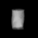
Negative-log display: 0–8
Accepted prediction
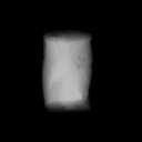
Negative-log display: 0–8
Hatching: no observations. Rust boundaries: fitted columns 60–67. Predictions outside the strip are excluded from the objective.
128 × 128 detector samples · 8 mm pitch · 1,024 × 1,024 mm detector extent · image top is +v. Display: −log((counts + 0.5) / open beam), 0–8. The pseudocount is absent from the Poisson objective. Termination: line search failed. The accepted pose is not stationary.
Accepted iterates and the unchanged stationarity test
- Orthogonal views
- Near-parallel views
- Restricted, low-count
- Original stationarity threshold
Geometric error at the recorded accepted poses
- Orthogonal views
- Near-parallel views
- Restricted, low-count
- RMS gate (1 mm)
Both plots retain the same three examples. Error uses 125 fixed mathematical probes at every recorded pose. Reference poses were disclosed after fitting, without guiding the solver or selecting an iterate.
All 136 application outcomes and numerical records · Sources, rights and display rules. CT anatomy is acquired. Attenuation assignments and radiographs are simulated.
Figure 11.4 retains all 40 historical outcomes, including the eight restricted cases that fail the geometric criterion. These are the original stopped fits, not additional converged runs of the revised example.
Prescribed starts and final geometric error
- Orthogonal
- Near-parallel
- Restricted, low-count
- RMS success threshold
Paired full-view registration errors
- Case 0
- Case 1
All 32 full-view fits passed: probe RMS ≤1 mm, maximum error ≤2 mm, rotation error ≤0.5°. All eight restricted fits failed. The 125 probes are mathematical points, not anatomical landmarks. Overlapping markers are listed separately below.
All 40 fits: pose errors and stopping tests
| Case / arrangement / noise / start | Initial RMS / mm | Final RMS / mm | Maximum / mm | Rotation / ° | Gradient norm |
|---|---|---|---|---|---|
| 0 / Orthogonal views / 0 / 0 | 4.9403 | 0.0179 | 0.0298 | 0.0138 | 1.866 |
| 0 / Near-parallel views / 0 / 0 | 4.9403 | 0.0145 | 0.0246 | 0.0099 | 0.1013 |
| 0 / Orthogonal views / 0 / 1 | 8.6206 | 0.0180 | 0.0299 | 0.0138 | 0.4486 |
| 0 / Near-parallel views / 0 / 1 | 8.6206 | 0.0145 | 0.0246 | 0.0099 | 0.3637 |
| 0 / Orthogonal views / 0 / 2 | 7.6250 | 0.0180 | 0.0298 | 0.0138 | 0.09378 |
| 0 / Near-parallel views / 0 / 2 | 7.6250 | 0.0145 | 0.0246 | 0.0099 | 0.1409 |
| 0 / Orthogonal views / 0 / 3 | 17.8341 | 0.0180 | 0.0298 | 0.0138 | 0.07825 |
| 0 / Near-parallel views / 0 / 3 | 17.8341 | 0.0145 | 0.0246 | 0.0099 | 0.02584 |
| 0 / Orthogonal views / 1 / 0 | 4.9403 | 0.0133 | 0.0206 | 0.0053 | 0.4154 |
| 0 / Near-parallel views / 1 / 0 | 4.9403 | 0.0176 | 0.0309 | 0.0094 | 1.411 |
| 0 / Orthogonal views / 1 / 1 | 8.6206 | 0.0133 | 0.0206 | 0.0053 | 0.1103 |
| 0 / Near-parallel views / 1 / 1 | 8.6206 | 0.0177 | 0.0310 | 0.0094 | 0.2947 |
| 0 / Orthogonal views / 1 / 2 | 7.6250 | 0.0132 | 0.0205 | 0.0052 | 1.566 |
| 0 / Near-parallel views / 1 / 2 | 7.6250 | 0.0178 | 0.0312 | 0.0094 | 0.3468 |
| 0 / Orthogonal views / 1 / 3 | 17.8341 | 0.0133 | 0.0206 | 0.0053 | 0.5080 |
| 0 / Near-parallel views / 1 / 3 | 17.8341 | 0.0177 | 0.0311 | 0.0094 | 0.4537 |
| 0 / Restricted, low-count / 0 / 0 | 4.9403 | 1.6679 | 2.6445 | 0.6520 | 0.01123 |
| 0 / Restricted, low-count / 0 / 1 | 8.6206 | 2.7570 | 4.2532 | 1.1191 | 0.01632 |
| 0 / Restricted, low-count / 0 / 2 | 7.6250 | 1.6686 | 2.6456 | 0.6521 | 0.01158 |
| 0 / Restricted, low-count / 0 / 3 | 17.8341 | 1.6703 | 2.6478 | 0.6524 | 0.005984 |
| 1 / Orthogonal views / 0 / 0 | 5.0912 | 0.0067 | 0.0108 | 0.0043 | 2.281 |
| 1 / Near-parallel views / 0 / 0 | 5.0912 | 0.0070 | 0.0131 | 0.0064 | 0.8148 |
| 1 / Orthogonal views / 0 / 1 | 8.7995 | 0.0067 | 0.0109 | 0.0043 | 0.3454 |
| 1 / Near-parallel views / 0 / 1 | 8.7995 | 0.0070 | 0.0131 | 0.0064 | 2.310 |
| 1 / Orthogonal views / 0 / 2 | 7.6751 | 0.0067 | 0.0109 | 0.0043 | 0.02352 |
| 1 / Near-parallel views / 0 / 2 | 7.6751 | 0.0070 | 0.0131 | 0.0064 | 1.325 |
| 1 / Orthogonal views / 0 / 3 | 17.8710 | 0.0067 | 0.0109 | 0.0043 | 0.08475 |
| 1 / Near-parallel views / 0 / 3 | 17.8710 | 0.0070 | 0.0131 | 0.0064 | 0.06669 |
| 1 / Orthogonal views / 1 / 0 | 5.0912 | 0.0107 | 0.0175 | 0.0095 | 0.1847 |
| 1 / Near-parallel views / 1 / 0 | 5.0912 | 0.0218 | 0.0344 | 0.0098 | 2.122 |
| 1 / Orthogonal views / 1 / 1 | 8.7995 | 0.0107 | 0.0176 | 0.0095 | 0.2892 |
| 1 / Near-parallel views / 1 / 1 | 8.7995 | 0.0218 | 0.0343 | 0.0098 | 0.2143 |
| 1 / Orthogonal views / 1 / 2 | 7.6751 | 0.0107 | 0.0175 | 0.0095 | 0.06192 |
| 1 / Near-parallel views / 1 / 2 | 7.6751 | 0.0218 | 0.0343 | 0.0098 | 0.09484 |
| 1 / Orthogonal views / 1 / 3 | 17.8710 | 0.0107 | 0.0175 | 0.0095 | 0.05459 |
| 1 / Near-parallel views / 1 / 3 | 17.8710 | 0.0219 | 0.0345 | 0.0098 | 0.4019 |
| 1 / Restricted, low-count / 0 / 0 | 5.0912 | 1.5336 | 2.3953 | 1.0941 | 0.01145 |
| 1 / Restricted, low-count / 0 / 1 | 8.7995 | 1.5654 | 2.5151 | 1.0559 | 0.03269 |
| 1 / Restricted, low-count / 0 / 2 | 7.6751 | 1.5341 | 2.3966 | 1.0940 | 0.01033 |
| 1 / Restricted, low-count / 0 / 3 | 17.8710 | 1.5655 | 2.5147 | 1.0560 | 0.002869 |
Every solve stopped with line_search_failed. Every final gradient norm exceeds the fixed 0.001 threshold. Reference transforms and two complete reserved views per fit were assessed after the accepted results were fixed.
All 136 application outcomes and numerical records · Sources, rights and display rules. CT anatomy is acquired. Attenuation assignments and radiographs are simulated.
The known volume has constrained every pose trial in this chapter. Chapter 12 removes that advantage: geometry is fixed, and the unknowns become the attenuation values themselves. The renderer stays recognisable. The space of plausible explanations becomes much larger.
References
- Otake, Yoshito, Wang, Adam S., Stayman, J. Webster, Uneri, Ali, Kleinszig, Gerhard, Vogt, Sebastian, Khanna, A. Jay, Gokaslan, Ziya L. and Siewerdsen, Jeffrey H. (2013). Robust 3D–2D image registration: application to spine interventions and vertebral labeling in the presence of anatomical deformation. Physics in Medicine and Biology, 58(23), 8535-8553. https://doi.org/10.1088/0031-9155/58/23/8535
- Gopalakrishnan, Vivek, Dey, Neel and Golland, Polina (2024). Intraoperative 2D/3D Image Registration via Differentiable X-ray Rendering. Proceedings of the IEEE/CVF Conference on Computer Vision and Pattern Recognition, 11662-11672. https://doi.org/10.1109/CVPR52733.2024.01108