Choosing the next view and where to spend the photons
Some measurements constrain the quantity we care about more than others. We use local uncertainty to compare feasible views and examine how exposure can be allocated to the task.
A registration can fit its first X-ray closely while leaving the object free to move along a poorly observed direction. Another image might resolve that uncertainty. Taking almost the same view again mostly provides more photons along directions already measured. Moving the C-arm incurs its own costs, and the angle with the prettiest derivative image may be physically inaccessible. We need to predict which feasible measurement will reduce uncertainty in the task we care about.
We will choose one additional view of the known attenuation volume used in Chapter 11, generate that view’s observation and fit the updated pose. The worked example completes the entire sequence. Across eight prescribed Poisson noise pairs, its selected view reduces mean squared target error by 71% against a nearly repeated 5° view at the same exposure. Every base and final fit reaches the numerical stopping tolerance and passes independent geometric and reserved-view checks. The complete recipe supplies the admitted CT-derived input and connects the canonical dpt.examples.acquisition_design selector to observation generation and registration.
The forward model and pose convention come from Chapter 11. Chapter 12 supplies the harder extension in which the unknown is a volume. We will keep track of the information available before each decision, because a policy that has already seen tomorrow’s X-ray tends to perform suspiciously well.
13.1 Define the task and the information available
Suppose the current data are and the next acquisition is described by : its source and detector geometry together with calibrated exposure settings. A decision rule can use the known volume, , the current pose estimate and a declared uncertainty model. It may render hypothetical measurements at candidate acquisitions. It cannot use their future measured pixel values.
For registration, the quantity of interest need not be an equally weighted combination of translation and rotation. A small rotation produces a larger displacement at a distant surgical target than near the rotation centre. We therefore supply object-frame target points and score their predicted world-coordinate variance. These points describe the task using anatomy already available to the policy. Withheld reference transformations are used later to measure error.
A fixed design chooses the entire sequence before seeing any new measurements. A sequential design chooses the next acquisition, receives its observation, updates the estimate and chooses again. The executable example implements one decision in the latter sequence. Its supplied current precision must describe uncertainty at that decision, including previous measurements exactly once. Adding their information again would reward the policy for counting its homework twice.
Figure 13.1 separates these inputs from the withheld evaluation reference. The same separation belongs in the file layout: the design case contains calibrated candidate predictions and the current state, while the later evaluation record supplies the selected measured image and independent reference.
13.2 Choose a task-specific design objective
Keep the pose chart fixed while comparing candidates. At the current transform , use dimensionless coordinates with positive diagonal scale matrix :
The first three entries of set translation scales in millimetres, and the remaining entries set rotation scales in radians. All derivatives in this section are evaluated at . Equation (13.1) is a local right update. A precision matrix expressed in another frame, at another chart centre or with different scales must be transformed before use.
For candidate , assume conditionally independent ideal counts . At positive means, the score contribution is . Its expectation is zero and its variance uses . Independence removes cross-pixel score covariances, giving the expected Fisher information
A large image derivative contributes little useful information if its noise is large or if it repeats an already well-observed parameter direction. For the primary model, let be the canonical optical depth and the fixed open-beam expectation. Since , equation (13.2) becomes
where has one row per pixel. This form avoids dividing by a count prediction that may round to zero. A genuinely zero supplied beam contributes zero information: no image of the object arrives along that ray. Correlated read noise, energy integration and shared calibration errors require their own likelihood. Independent Poisson weighting does not become appropriate merely because an image came from an X-ray detector.
Let the current pose distribution be approximated locally by a Gaussian with positive-definite precision in this same chart. Adding expected information gives
Equation (13.4) predicts local covariance using expected likelihood curvature. It is neither an exact posterior covariance for every possible future image nor a guarantee that the registration solver will find the intended pose. The current uncertainty can already include earlier acquisitions. A numerical damping matrix inserted into an optimiser is not automatically a defensible .
For an object-frame target , differentiating its world position under equation (13.1) gives
Here . The translation part of moves every target alike, while its rotation part retains the distance and direction from the object origin. Averaging target-position variance gives the scalar criterion
Its units are square millimetres. This predicts spread, not squared error including unknown bias. Listing 13.1 computes the target derivatives and scores this criterion through Cholesky solves. The scorer requires strictly positive-definite current precision and reports an error when that assumption fails. It adds no identity matrix to supply missing precision.
def target_jacobians(np: Any, pose: RigidTransform, targets: Any, scales: Any) -> Any:
    """Return d(world target)/dz in mm for T_WO exp((S z)^) at z=0."""
    rotation = np.asarray(pose.rotation, dtype=np.float64).reshape(3, 3)
    result = np.empty((len(targets), 3, 6), dtype=np.float64)
    for index, (x, y, z) in enumerate(targets):
        skew = np.asarray([[0.0, -z, y], [z, 0.0, -x], [-y, x, 0.0]])
        result[index, :, :3] = rotation
        result[index, :, 3:] = -rotation @ skew
    result *= scales[None, None, :]
    if not np.isfinite(result).all():
        raise NumericalError("target derivatives exceed FP64; check target coordinates and scales")
    return result


def target_variance(
    np: Any, precision: Any, target_jacobian: Any, maximum_condition: float
) -> tuple[float, Any, float]:
    """Mean target-position variance in mm², without forming an inverse to score."""
    if not np.isfinite(precision).all():
        raise NumericalError("pose precision is non-finite; discard this candidate score")
    values = np.linalg.eigvalsh(precision)
    if values[0] <= 0 or values[-1] / values[0] > maximum_condition:
        raise NumericalError(
            "pose precision must be positive definite and within maximum_precision_condition; "
            "check the stated uncertainty and parameter scales, without adding numerical jitter"
        )
    factor = np.linalg.cholesky(precision)
    right = target_jacobian.reshape(-1, 6).T
    whitened = np.linalg.solve(factor, right)
    if not np.isfinite(whitened).all():
        raise NumericalError(
            "target covariance solve exceeds FP64; check the precision and chart scales"
        )
    # hypot scales its sum of squares; individual products must not underflow
    # before they contribute to an otherwise representable total variance.
    normalisation = math.sqrt(len(target_jacobian))
    root_variance = math.hypot(*(float(value) / normalisation for value in whitened.flat))
    variance = root_variance * root_variance
    if not math.isfinite(variance) or variance <= 0:
        raise NumericalError(
            "positive target-position variance is outside FP64 range; check the stated "
            "uncertainty and physical units, or use a range-preserving score representation"
        )
    inverse_factor = np.linalg.solve(factor, np.eye(6))
    covariance = inverse_factor.T @ inverse_factor
    if not np.isfinite(covariance).all() or bool((np.diag(covariance) <= 0).any()):
        raise NumericalError(
            "local covariance is outside FP64 range; check the precision and chart scales "
            "before exporting this candidate"
        )
    return variance, covariance, float(values[-1] / values[0])
Nuisance parameters can substantially change the ranking. If describes uncertain calibration and the joint precision is partitioned into pose and nuisance blocks, the marginal pose precision is the Schur complement , assuming the required positive definiteness. Holding nuisance parameters fixed instead uses the pose block directly and can understate uncertainty. Our example makes that restriction explicit: acquisition calibration and attenuation are fixed, and only pose is uncertain.
13.3 Separate candidate selection from continuous optimisation
For a finite eligible set , the decision is simply . Score every candidate against the same current precision, pose and targets. Do not update the current precision after scoring a hypothetical candidate, because that would make the answer depend on enumeration order. Exact score ties in the example prefer lower cost, then the candidate name.
Finite enumeration needs derivatives with respect to pose at each fixed geometry. The library already exports these. Continuous optimisation of source position or detector orientation is a different implementation task: differentiating with respect to generally needs derivatives of both the mean and its pose Jacobian, including mixed pose–acquisition derivatives. The current projector supplies neither acquisition-geometry adjoints nor higher derivatives. Repeated calls to an existing first-order VJP do not establish either capability.
A criterion that includes a reconstruction solve adds another dependency. Differentiating a fixed number of solver iterations gives a derivative of that algorithm. Implicit differentiation instead uses an equation characterising the solution and requires appropriate local uniqueness, regularity and convergence. These quantities need not agree for an unfinished solve or at an active-set change. Holding the current estimate fixed does not differentiate its dependence on the acquisition. Record that approximation explicitly.
13.4 Restrict choices to feasible acquisitions
The candidate set should come from an imaging-system specification. Source and detector positions must respect working distance, angular travel and detector coverage. A reachable endpoint can still require a motion path that collides with equipment. Exposure settings may be discrete, and moving to a candidate may consume more time than taking its image. Geometry and movement costs therefore belong to each candidate record.
The example accepts candidates already assessed for feasibility and requires a description of that assessment. It checks the supplied ray geometry and a scalar acquisition budget, but it does not perform collision detection or certify a motion path. Figure 13.2 shows an illustrative endpoint constraint with excluded configurations marked separately. A high information score cannot disguise an unusable view.
A candidate’s open-beam array specifies the detector-incident expectation under that candidate’s calibrated source setting. If source motion changes distance or coverage, reusing the previous array without recalibration changes the assumed experiment. The JSON case binds every supplied array to its units, source hash and redistribution rights. For a cost expressed as expected detector photons, the code checks that the stated cost equals the open-beam sum in the absence of the object. This budget differs from the transmitted count sum.
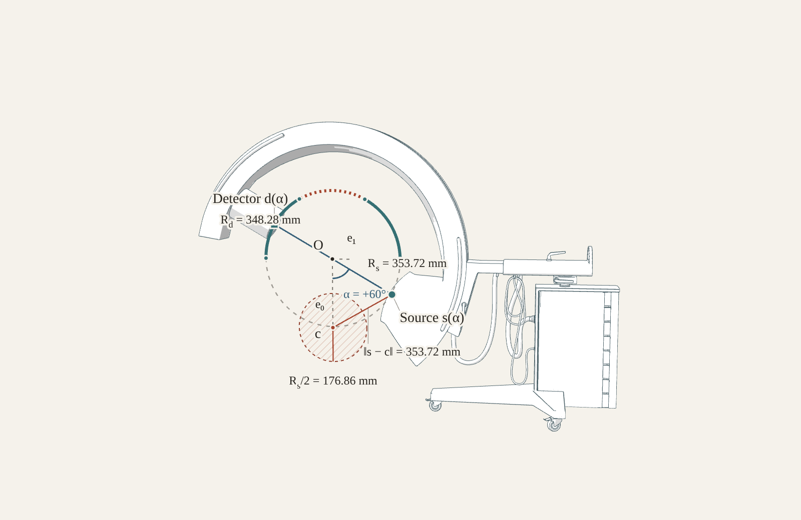
The annotated C-arm loads when this figure comes into view.
- Allowed detector endpoint
- Source-clearance exclusion
- Outside candidate domain
At +60°: source clearance 353.72 mm, detector configuration allowed.
relative to O, with .
Allowed: .
Model-world distances: ,. . The ±90° candidate domain and point-clearance disk are illustrative. They do not specify device travel or a collision-free path.
Use the angle slider to inspect the endpoint constraint. Camera orbiting changes only the view.13.5 Choose a second view for registration
The application case provides the known attenuation field, current pose and local precision, with targets defined in object coordinates. It supplies candidate geometries and calibrated beams, but no future radiographs. The evaluator uploads the field once, uses one CUDA stream for Warp and PyTorch, and constructs each candidate’s depth Jacobian through projection_pose_sensitivities.
The exported derivative uses physical millimetres and radians. Multiplying its columns by the supplied scales converts it to in equation (13.3). On the GPU, the FP64 path forms directly from retained optical depth; the FP32 path uses the canonical log-transmission output. FP64 exponential weighting preserves a wider range than deriving weights from stored FP32 counts. The weighted Jacobian then reduces to a information matrix through a CUDA matrix product. Only that matrix and a few scalar diagnostics return to the host.
Listing 13.2 shows the complete candidate calculation. One candidate needs the exported Jacobian and a weighted copy, together bytes, plus optical-depth, beam and statistical scratch. PyTorch allocates intermediate tensors during this bounded offline calculation. max_candidate_pixels bounds the retained detector-sized work, and the stream completes before its temporary owners are released.
def candidate_information(
    *,
    np: Any,
    torch: Any,
    ctx: Any,
    grid: GridSpec,
    geometry: DetectorGeometry,
    attenuation: Any,
    pose: Any,
    beam_host: Any,
    scales: Any,
    samples_per_ray: int,
    precision: Literal["float32", "float64"] = "float32",
    integration: Literal["midpoint", "cell_gauss"] = "midpoint",
) -> tuple[Any, dict[str, Any]]:
    """Use canonical depth derivatives and an FP64 CUDA Fisher reduction.

    Preparation allocates one candidate's O(6P) Jacobian and weighted copy.
    Torch views alias Warp storage on the same CUDA stream. There is no
    per-pixel Python loop and no image/Jacobian download. This is an offline
    candidate evaluation, not a captured or profiled optimisation hot path.
    """
    wp, pixels = ctx.wp, geometry.pixels
    try:
        projection = prepare_projection(
            grid,
            geometry,
            ProjectionSpec(samples_per_ray, precision=precision, integration=integration),
            device=str(ctx.device),
            stream=ctx.stream,
        )
        transmission = (
            prepare_transmission(
                TransmissionSpec(beam="none"),
                max_pixels=pixels,
                device=str(ctx.device),
                stream=ctx.stream,
            )
            if precision == "float32"
            else None
        )
        with ctx.scope():
            beam = wp.array(beam_host.reshape(-1), dtype=wp.float32, device=ctx.device)
            depth = wp.empty(pixels, dtype=projection.dtype, device=ctx.device)
            log_transmission = wp.empty(
                pixels if precision == "float32" else 0, dtype=wp.float32, device=ctx.device
            )
            ones = wp.ones(pixels, dtype=projection.dtype, device=ctx.device)
            jacobian = wp.empty(6 * pixels, dtype=wp.float64, device=ctx.device)
        project_optical_depth(
            attenuation,
            pose,
            workspace=projection,
            out_L=depth,
            stream=ctx.stream,
        )
        if transmission is not None:
            transmit(
                depth,
                out_log_T=log_transmission,
                workspace=transmission,
                stream=ctx.stream,
            )
        projection_pose_sensitivities(
            attenuation,
            pose,
            ones,
            out_jacobian=jacobian,
            workspace=projection,
            stream=ctx.stream,
        )
        beam_tensor = wp.to_torch(beam)
        log_mean = beam_tensor.to(dtype=torch.float64).log_()
        if precision == "float64":
            log_mean.sub_(wp.to_torch(depth))
        else:
            log_mean.add_(wp.to_torch(log_transmission))
        illuminated = beam_tensor > 0
        # A zero supplied beam carries no information. Positive means outside
        # the normal FP64 range are rejected; no tail, floor or pixel is hidden.
        log_tiny = math.log(float(np.finfo(np.float64).tiny))
        if bool((illuminated & (log_mean < log_tiny)).any().item()):
            raise NumericalError(
                "a positive candidate count mean is below normal FP64 range; "
                "use a range-preserving design implementation before ranking this case"
            )
        root_mean = log_mean.mul_(0.5).exp_()
        depth_jacobian = wp.to_torch(jacobian).reshape(pixels, 6)
        weighted = depth_jacobian.clone()
        weighted.mul_(scales).mul_(root_mean[:, None])
        if not bool(torch.isfinite(weighted).all().item()):
            raise NumericalError("weighted pose derivatives exceed FP64; discard this candidate")
        if bool(((depth_jacobian != 0) & illuminated[:, None] & (weighted == 0)).any().item()):
            raise NumericalError(
                "a nonzero weighted derivative underflowed; discard this candidate"
            )
        magnitude = weighted.abs()
        minimum = math.sqrt(float(np.finfo(np.float64).tiny))
        maximum = math.sqrt(float(np.finfo(np.float64).max) / (6.0 * pixels))
        if bool((((magnitude > 0) & (magnitude < minimum)) | (magnitude > maximum)).any().item()):
            raise NumericalError(
                "candidate Fisher products exceed the declared FP64 accumulation range; "
                "rescale the pose chart or use a range-preserving reduction"
            )
        # Weighted depth derivatives give J_L^T diag(lambda) J_L directly.
        # Avoid a division by rounded, potentially zero count predictions.
        information = weighted.T @ weighted
        result = information.cpu().numpy().copy()
        if not np.isfinite(result).all():
            raise NumericalError("candidate information is non-finite; discard this score")
        diagnostics = {
            "pixels": pixels,
            "precision": precision,
            "integration": integration,
            "zero_beam_pixels": int((~illuminated).sum().item()),
            "omitted_positive_beam_pixels": 0,
            "jacobian_and_weighted_copy_bytes": 2 * 6 * pixels * 8,
            "fisher_reduction": "FP64 CUDA; only the 6 by 6 information matrix is downloaded",
        }
        return 0.5 * (result + result.T), diagnostics
    finally:
        # Warp owners and the host beam must survive every pending shared-stream operation.
        wp.synchronize_stream(ctx.stream)
Numerical range remains part of the method. A dark pixel with a supplied zero beam contributes exactly zero. For illuminated pixels, the example rejects means below the normal FP64 range and rejects weighted derivative products outside its declared accumulation range. It adds no count floor and omits no positive-beam tail to obtain a ranking. Such a rejection calls for a more capable numerical reduction or a better-scaled chart, followed by independent verification. The actual depth and depth Jacobian remain the discretised quantities produced by the canonical projector.
Listing 13.3 adds each candidate’s information to the same current precision, computes the target criterion and records threshold-defined local Fisher rank. Rank depends on the stated tolerance and parameter scaling. A view can reduce variance along an existing direction without increasing rank, so rank alone is not the selection rule.
                for candidate in eligible:
                    information, diagnostics = candidate_information(
                        np=np,
                        torch=torch,
                        ctx=ctx,
                        grid=grid,
                        geometry=candidate["geometry"],
                        attenuation=attenuation,
                        pose=pose_device,
                        beam_host=candidate["beam"],
                        scales=scales_device,
                        samples_per_ray=samples,
                        precision=cfg.get("precision", "float32"),
                        integration=cfg.get("integration", "midpoint"),
                    )
                    variance, covariance, condition = target_variance(
                        np, prior + information, target_derivatives, maximum_condition
                    )
                    eigenvalues = np.linalg.eigvalsh(information)
                    largest = float(eigenvalues[-1])
                    if eigenvalues[0] < -rank_tolerance * max(largest, np.finfo(np.float64).tiny):
                        raise NumericalError(
                            "candidate Fisher matrix is indefinite beyond rank tolerance"
                        )
                    rank = int(np.count_nonzero(eigenvalues > rank_tolerance * largest))
                    rows.append(
                        {
                            "name": candidate["name"],
                            "cost": candidate["cost"],
                            "mean_target_variance_mm2": variance,
                            "local_fisher_rank": rank,
                            "posterior_precision_condition": condition,
                            "diagnostics": diagnostics,
                        }
                    )
                    matrices.append(information)
                    covariances.append(covariance)
                # Exact score ties prefer the smaller stated cost, then the name.
                selected = min(
                    rows,
                    key=lambda row: (row["mean_target_variance_mm2"], row["cost"], row["name"]),
)The worked sequence begins with a 0° image at an open-beam expectation of 1,000 photons per pixel. Once that base fit has converged, the selector compares 5°, 30°, 60° and 90° at the same exposure. The base view’s Fisher matrix at its accepted pose supplies , so the first image enters the uncertainty calculation once, before each candidate’s information is added. The calculation uses the exact cell integration and FP64 arithmetic checked in Chapter 11 for both the current information and each candidate. The task points are the eight corners with object-frame coordinates ±40 mm; the later geometric evaluation uses those very same points.
In the first noise replicate, the selector chooses 60°, with predicted mean target variance 0.001325 mm². Moving farther to 90° gives a larger value, 0.001946 mm². Angular separation alone therefore does not explain this ranking: the criterion measures how each view constrains these targets through the supplied anatomy at the current pose. After recording the choice, the driver draws its count image and refits the pose. Figure 13.3 compares that prediction with the realised errors across all eight pairs.
The first view choice
- Other candidates
- Selected view
All eight recovery outcomes
- Near-parallel 5°
- Selected view
The selected view reduces mean squared target error by 71% relative to the near-parallel view. 2 of the 8 pairs have higher error after selection: the criterion predicts an average over possible count images, while each pair receives one noise realisation. This controlled example demonstrates the average benefit; it does not promise to beat every well-chosen fixed view.
| Quantity | Result | Criterion |
|---|---|---|
| Completed solves | 25 / 25 stationary, geometrically accurate and reserved-view checks passed | Every prescribed solve passes |
| Selected mean squared target error | 0.0013347 mm² | ≤ 75% of near-parallel baseline |
| Near-parallel mean squared target error | 0.0046812 mm² | Same exposure and solver |
| Selected / baseline | 0.2851 | ≤ 0.75 |
| Paired descriptive 95% upper bound | -0.0005937 mm² | Below zero |
Reproduction and recorded data
The 5° baseline deliberately spends its second exposure on almost the same view. It makes the value of measuring a different direction visible in a small complete example. This result does not establish superiority over a well-chosen fixed orthogonal view. When the first image admits distant plausible poses, a Gaussian around one estimate can also miss those alternatives. An independently specified pose ensemble or expected information gain over a multimodal posterior would address that different approximation.
13.6 Design views for reconstruction
An attenuation volume replaces the six pose coordinates with perhaps millions of unknown coefficients. The design question still needs a task: variance of a regional average, visibility of a specified feature or reconstruction error under a declared prior ensemble. Summing uncertainty equally over all voxels can spend acquisitions on parts of the field that do not matter to that task.
A local approximation has a precision operator of the form
where describes current local precision and follows the candidate’s measurement model. A dense volume covariance would require quadratic storage. Instead, an implementation could apply precision to vectors and solve for the covariance action needed by a small set of task functionals. For a linear task , the local variance is , and a linear solve can obtain it without constructing the inverse.
Equation (13.7) describes an extension, not a capability exercised by the registration example. A matrix-free implementation needs compatible Jacobian-vector and transpose products, a declared regulariser Hessian, and independently checked solver tolerances. The available volume VJP provides the transpose action but does not by itself provide the entire design calculation. Nonnegativity constraints and changes of active set further affect a local Gaussian approximation.
Burger and colleagues develop sequential Bayesian projection design with Gaussian priors and additive Gaussian noise, including criteria based on posterior covariance and information. Their numerical study concerns two-dimensional parallel-beam tomography. It gives a concrete precedent for updating projection choices as data arrive, but the three-dimensional Poisson pose calculation here has its own likelihood and geometry. [38]
Compare reconstruction policies at the same measurement budget and include the time spent deciding which view to take. An expensive design search can be appropriate for a costly acquisition. It can also become a remarkably elaborate method of avoiding the next reconstruction. Spectral-channel choices add the calibrated response and material-identifiability conditions developed in §12.6. They cannot be ranked from geometric coverage alone.
13.7 Allocate exposure and state the budget correctly
Under a fixed spectrum and linear independent-count model, suppose a relative exposure scales the expected counts as . The depth Jacobian stays fixed, so
Information grows linearly in this model, but the resulting target variance generally does not, because it depends on the inverse of the sum of prior and measurement information. Detector saturation, spectral changes or exposure-dependent processing invalidate the simple scaling. Each requires a forward and noise model that follows the actual control setting.
The example permits several candidate records with the same geometry and different calibrated beam/cost pairs. This evaluates discrete exposure alternatives for one next view. A multi-view allocation would instead choose exposures jointly under a total budget and per-view bounds, and would need to retain the dependence of its criterion on every allocation. Movement time can be included only when the cost is defined consistently with the current system state.
Expected detector photons, tube-current–time product in mAs and acquisition time in seconds are different budgets. None is absorbed dose. A dose-constrained extension must define whose absorbed energy per unit mass is being constrained and use a separately validated deposition model that accounts for spectrum, geometry and material. The number of Monte Carlo histories used to estimate a prediction is a computational setting, not the exposure given to a subject.
The worked comparison holds expected open-beam photons fixed and changes the second angle. It therefore demonstrates an angular decision at equal exposure. An exposure-allocation curve would need several controlled photon populations and must retain that axis label, even if “dose reduction” would fit rather nicely in the abstract.
13.8 Complete and check the acquisition sequence
Run the Chapter 11 recipe through to summary.json. After the orthogonal registration, the driver performs eight base fits and sixteen paired refits. Within each pair, selection and the 5° baseline share the same first image, so their comparison holds that image’s noise fixed. The driver records the selected angle before generating its observation. If both policies request the same future view, they receive the same observation; different acquisitions use separately keyed random streams.
            for replicate in range(replicates):
                beam = protocol["acquisition"]["base_and_candidate_open_beam_per_pixel"]
                base_id = _observation(
                    record, public, means, protocol, 0.0, beam, 2, replicate, seed
                )
                base = _fit(
                    known_root,
                    output,
                    public,
                    protocol,
                    f"base-{replicate:02d}",
                    [base_id],
                    RigidTransform(),
                    device,
                )
                accepted = rigid(base["pose_object_to_world"])
                decision_path = output / f"decision-{replicate:02d}"
                selection = rank_design(
                    known_root,
                    output,
                    public,
                    protocol,
                    {
                        "angles": protocol["acquisition"]["candidate_angles_degrees"],
                    },
                    accepted,
                    decision_path,
                    device,
                )
                # Selection is on disk before either future count image exists.
                record.write_json(f"decision-{replicate:02d}-binding.json", selection)
                pair = {"replicate": replicate, "base": base, "selection": selection}
                for policy, angle in (
                    ("selected", selection["selected_angle"]),
                    ("near_parallel", protocol["acquisition"]["fixed_view_degrees"]),
                ):
                    future_id = _observation(
                        record, public, means, protocol, angle, beam, 3, replicate, seed
                    )
                    pair[policy] = _fit(
                        known_root,
                        output,
                        public,
                        protocol,
                        f"{policy}-{replicate:02d}",
                        [base_id, future_id],
                        accepted,
                        device,
                    )
results.append(pair)The frozen configuration fixes the eight noise replicates, exposure, candidate set, probe locations and success criteria. The input anatomy is intentionally known for this instructional exercise. Evaluation transforms and the reserved 45° and 135° view means are kept out of fitting and ranking. After all fits have finished, the evaluator measures target error and checks predictions in both reserved views.
Every one of the 25 solves, including the initial Chapter 11 registration, reaches the unchanged scaled-gradient threshold of 0.001 and passes its independent checks. The selected policy’s mean squared target error is 0.001335 mm², compared with 0.004681 mm² for the near-parallel baseline: a ratio of 0.2851, below the declared 0.75 requirement. The paired mean difference is −0.003347 mm², with a descriptive 95% t-interval upper endpoint of −0.000594 mm². This interval summarises eight prescribed noise pairs on one anatomy; it is not an estimate of clinical benefit across patients.
In two of the eight pairs, the selected view produces a larger target error than the 5° baseline. The Fisher criterion predicts variance averaged over possible future count images, while each refit receives one new noisy image alongside the shared base image. A view with lower predicted variance can therefore give the worse result in an individual pair. The mean improvement includes both reversals, without requiring every noisy observation to be unusually obliging.
To extend the experiment, change one declared setting at a time and write a new record. Add an orthogonal fixed baseline to ask a harder comparison question, or restrict the candidate angles to study accessibility. A new anatomy, calibration error or a poor initial pose can change the ranking and its reliability. Keep those results separate from the supplied worked example, with every attempted outcome retained.
What the earlier policy comparison could not establish
The earlier study below tested selected, fixed and random policies across two CT-derived phantoms. Its 96 base and policy fits used assigned attenuation and simulated observations. All pass the geometric criterion, but none meets the unchanged stationarity threshold. The registration replay in Chapter 11 identified precision loss and midpoint integration artefacts that can produce these premature stops. Until the downstream solver completes, a policy comparison mixes the view’s information with the behaviour of an unfinished optimisation.
Figure 13.4 retains those original outcomes. The paired noise intervals do not establish a consistent advantage over the fixed policy. This is why the main exercise now completes every solve and uses a clearly stated near-parallel baseline. It does not relabel the historical results as successful optimisation.
Predicted local variance before acquisition
First prescribed replicate. Selection minimises predicted variance at eight fixed object-frame corners, using the nonstationary first-view pose. Evaluation uses 125 separate mathematical probes.
| Additional angle | Predicted variance / mm² | Choice |
|---|---|---|
| -90° | 0.00225 | — |
| -60° | 0.00191 | — |
| -30° | 0.00244 | — |
| 30° | 0.00197 | — |
| 60° | 0.00171 | Selected |
| 90° | 0.00199 | — |
| Additional angle | Predicted variance / mm² | Choice |
|---|---|---|
| -90° | 0.00193 | — |
| -60° | 0.00166 | Selected |
| -30° | 0.00248 | — |
| 30° | 0.00203 | — |
| 60° | 0.00176 | — |
| 90° | 0.00189 | — |
Measured error after registration
Selection chose +60° for case 0 and −60° for case 1, while the fixed policy used +90°. Plots show achieved errors, not predicted variances.
Case 0: broad candidate set
- Selected
- Fixed
- Random
Case 1: broad candidate set
- Selected
- Fixed
- Random
Matching angles share observations within each replicate, so markers may overlap. Both plots use the same probes and scale. Lower predicted variance did not consistently reduce achieved error.
| Case | Comparison | Pairs | Mean difference | Descriptive 95% interval |
|---|---|---|---|---|
| 0 | fixed | 8/8 | -0.00492 | -0.02012 to 0.01056 |
| 0 | random | 8/8 | -0.00706 | -0.01702 to -0.00055 |
| 1 | fixed | 8/8 | -0.00544 | -0.01414 to 0.00295 |
| 1 | random | 8/8 | -0.00340 | -0.01264 to 0.00450 |
Negative differences favour selection. Percentile bootstrap intervals describe paired noise within each phantom, not population performance across CTs. Both selected-versus-fixed intervals include zero.
Before and after: all policy means and reserved-view errors
| Case | Policy | Fits | Mean probe RMS / mm | Mean reserved-view standardised RMS |
|---|---|---|---|---|
| 0 | Before additional view | 8 | 0.10334 | 0.03676 |
| 0 | selected | 8 | 0.04093 | 0.01521 |
| 0 | fixed | 8 | 0.04585 | 0.01800 |
| 0 | random | 8 | 0.04799 | 0.01644 |
| 1 | Before additional view | 8 | 0.07816 | 0.02643 |
| 1 | selected | 8 | 0.03592 | 0.01242 |
| 1 | fixed | 8 | 0.04136 | 0.01358 |
| 1 | random | 8 | 0.03932 | 0.01427 |
Reserved-view RMS compares prediction with the independent generating mean on two excluded views, scaled pixelwise by the generating Poisson SD. The table averages per-fit RMS values, not noisy-observation residuals.
Every additional view costs 16,384,000 expected detector-incident photons. Including the initial view gives 32,768,000. This is a photon-population budget, not absorbed dose. All 64 base and policy fits passed the geometric gates and ended with line_search_failed. None met the gradient threshold of 0.001.
All outcomes, paired replicates and 24 decisions · Sources, rights and display rules. TCIA CT-ORG cases 0 and 1, with assigned monochromatic attenuation and simulated radiographs.
Figure 13.5 shows the earlier restricted-angle comparison at fixed exposure. Under the constrained candidate set, selection produces a higher mean geometric error for case 0. The recorded evidence does not separate local covariance approximation, candidate restrictions and unfinished fitting sufficiently to assign that increase to one cause. Treat it as a diagnostic example to rerun after the numerical checks pass, rather than evidence that the selector improves this restricted case.
Measured error after registration
Selection chose +30° in both cases, while the fixed policy used +15°. Plots show achieved errors, not predicted variances.
Case 0: constrained candidate set
- Selected
- Fixed
- Random
Case 1: constrained candidate set
- Selected
- Fixed
- Random
Matching angles share observations within each replicate, so markers may overlap. Both plots use the same probes and scale. Lower predicted variance did not consistently reduce achieved error.
| Case | Comparison | Pairs | Mean difference | Descriptive 95% interval |
|---|---|---|---|---|
| 0 | fixed | 4/4 | 0.00756 | -0.01286 to 0.02915 |
| 0 | random | 4/4 | -0.00285 | -0.00780 to -0.00017 |
| 1 | fixed | 4/4 | -0.00201 | -0.01734 to 0.01333 |
| 1 | random | 4/4 | 0.00227 | -0.01046 to 0.01333 |
Negative differences favour selection. Percentile bootstrap intervals describe paired noise within each phantom, not population performance across CTs. In case 0 the selected policy has a higher mean error than the fixed view.
Before and after: all policy means and reserved-view errors
| Case | Policy | Fits | Mean probe RMS / mm | Mean reserved-view standardised RMS |
|---|---|---|---|---|
| 0 | Before additional view | 4 | 0.08324 | 0.02975 |
| 0 | selected | 4 | 0.05170 | 0.01768 |
| 0 | fixed | 4 | 0.04415 | 0.01689 |
| 0 | random | 4 | 0.05455 | 0.01763 |
| 1 | Before additional view | 4 | 0.08849 | 0.03495 |
| 1 | selected | 4 | 0.04454 | 0.01539 |
| 1 | fixed | 4 | 0.04654 | 0.01841 |
| 1 | random | 4 | 0.04227 | 0.01699 |
Reserved-view RMS compares prediction with the independent generating mean on two excluded views, scaled pixelwise by the generating Poisson SD. The table averages per-fit RMS values, not noisy-observation residuals.
Every additional view costs 16,384,000 expected detector-incident photons. Including the initial view gives 32,768,000. This is a photon-population budget, not absorbed dose. All 32 base and policy fits passed the geometric gates and ended with line_search_failed. None met the gradient threshold of 0.001.
All outcomes, paired replicates and 24 decisions · Sources, rights and display rules. TCIA CT-ORG cases 0 and 1, with assigned monochromatic attenuation and simulated radiographs.
13.9 A closing word
Volume I ends with a calculation that can help choose its next measurement. We began with photon survival through a slab. Reaching this decision has required a working renderer and derivatives that can guide an inverse calculation. The complete examples now recover unknown parameters from simulated observations and check the returned solutions against independent references. It is quite a lot of machinery for choosing another X-ray, but we can now account for what the machinery does.
That gives us a practical starting point for a problem of our own. Changing the unknown from a pose to a material field has already shown how much of the forward calculation can survive a very different inverse problem. Its physical assumptions remain visible, so we can decide what a new application actually requires us to change. A more elaborate representation can then be a deliberate modelling choice, with a calculation we understand beneath it.
Volume II is planned to cover neural representations and learned methods, and Volume III to develop volume reconstruction further. Those subjects have a place to begin in the forward model we have built here. Thank you for working through the physics and code with me. I hope that, when you next encounter a difficult imaging problem, a working calculation feels within reach.
References
- Burger, M, Hauptmann, A, Helin, T, Hyvönen, N and Puska, J-P (2021). Sequentially optimized projections in x-ray imaging. Inverse Problems, 37(7), 075006. https://doi.org/10.1088/1361-6420/ac01a4